4 Step by Step to Make Excel 3-D Pie Charts

How to create 3-D Pie-Charts in Excel

For creating a 3-D Pie-chart, follow these steps.

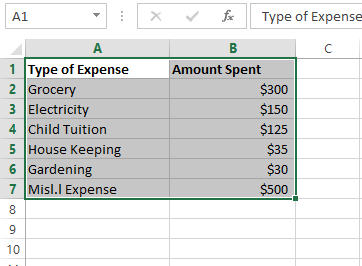
Step 1:

Select the data that you want to create a pie chart for. We have dummy data for home expenditures as shown below:

Step 2:

Go to Insert Tab in the Ribbon and select “Recommended Charts”

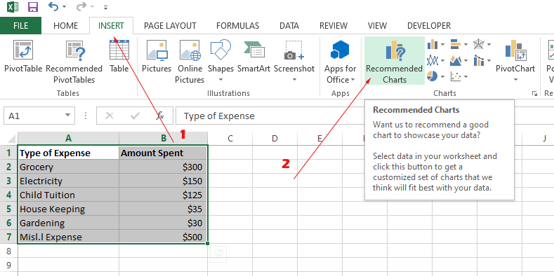
You may also select "Pie Chart" from the small icon adjacent to "Recommended Charts".

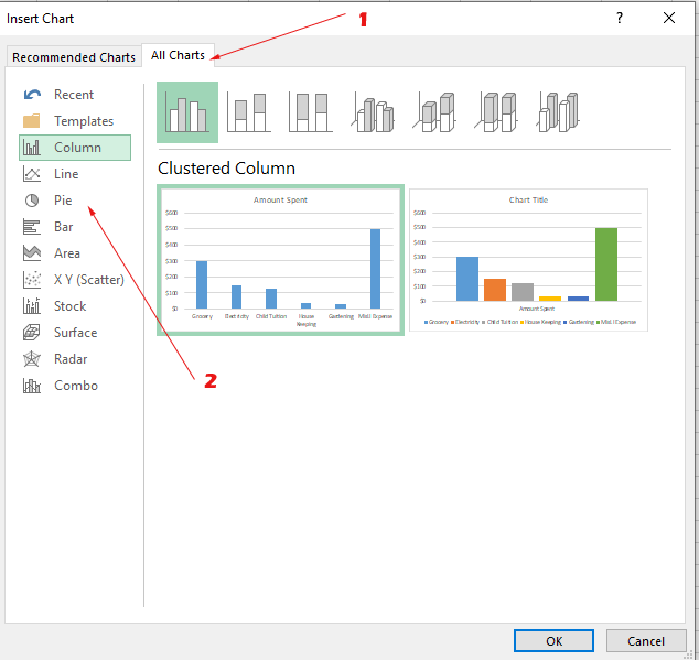
Step 3:

In the “Insert Chart” dialog, select “All Charts” and click on “Pie” as below:

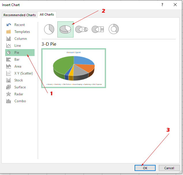
Step 4:

Under the “All Charts” tab for Pie, select “3-D Pie” and press the Ok button:

Result:

As you press Ok, it will create a Pie chart for the selected data as shown below:

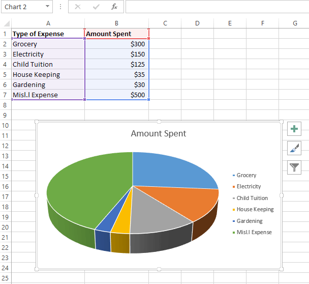
There you can see, Amount spent, which is our second column displayed as legend entries. Whereas, the first column is “Horizontal Axis Labels”.

Your second column should contain corresponding values to the first column towards the left.

Or you may set those ranges as shown in an example later.

How to display values/data table in the pie chart

You can see in the above result that no value is displayed in the chart. Instead, the “pies” size represents which Expense Type is more than others.

To display the amount (or any other figures in your sheet), follow these steps.

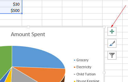
Step 1:

Select Pie chart and click on the + sign as shown below:

Step 2:

There, “Chart Elements” will display with two checked options and another unchecked.

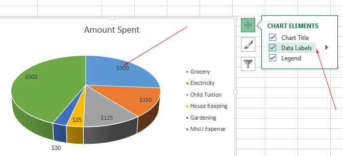
Check the “Date Labels” option and it should immediately display the Amount Spent values in their respective pies as shown in the above graphic.

Similarly, you may check/uncheck the other options like hiding the chart title and legends.

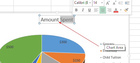
Changing the 3-D Pie chart title

The default title is the column header for the chart title. In our case, it took “Amount Spent”.

In order to change it, just click on the title and you can see a cursor allowing you to remove/edit the existing one:

Choosing the style of 3-D Pie chart

You may change the above-created default style of the Pie-chart easily.

Excel has many options to choose from. Follow this to choose a style of your choice or that best meets your needs.

Step 1:

Select a 3-D Pie chart that you created.

Step 2:

Click on the “Brush”

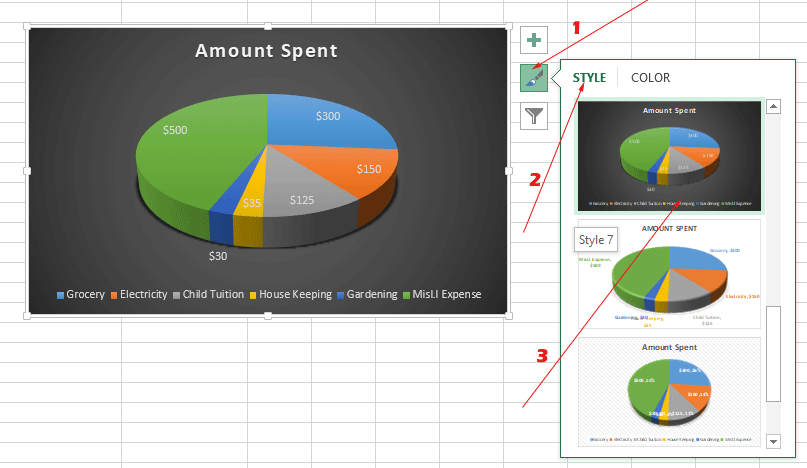
Under the STYLE, you can see available styles for 3-D pie charts.