Excel Drop-down List
In this tutorial, we will show you how to create a drop-down list in Excel that only shows values that you set along with an example of allowing users selecting a value from the available drop-down list plus writing their own.
A little about Excel Drop-down List
Having a drop-down list can be particularly useful if an Excel sheet is created by one and used by others.
In that case, you may limit the users to selecting a pre-given list of values in a cell.
Optionally, you may facilitate users for selecting a value from the available list along with adding new values that do not exist in the list.
In this tutorial, I will show you how to create a drop-down list in Excel that only shows values that you set along with an example of allowing users to select a value from the available drop-down list plus writing their own.
How to create a drop-down list in Excel?
Follow these steps for creating a drop-down list.
First, you have to create the source for the drop-down list. For that, you may write the drop-down list items on the same sheet or another sheet.
For the demo, I am writing the items on the same sheet that will appear in the drop-down. See the image below:
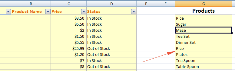
You can see that these are G2 to G10 cells that will act as the data source for the drop-down. Step 4 shows how to use it.
Select the cells where you want to create a drop-down as shown below:
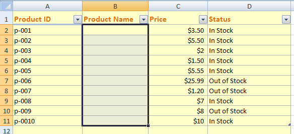
So in the end, the drop-down will appear from B2 to B11 cells in our example.
Go to the “Data” in the ribbon and locate the “Data Validation” group.
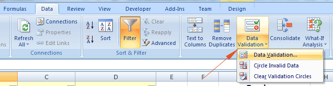
Click on the “Data Validation" option that should open the pop-up window.
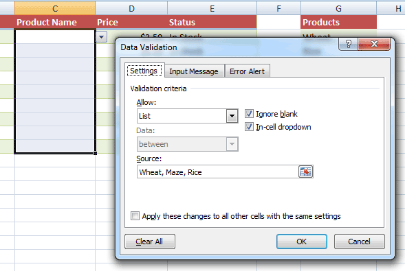
In the popup window, the Settings tab should already open. Under the “Validation Criteria”, click on the “Allow” drop-down and select the “List” option.
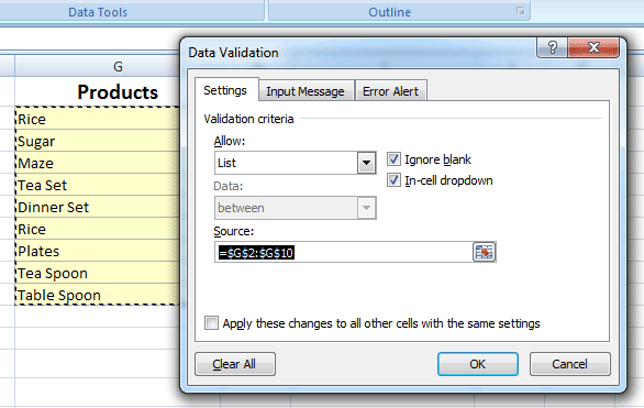
There you can also see the “Source” option. Click on the source textbox and select the cells in the sheet that we created for drop-down values i.e. G2 to G10 cells.
Press the OK button and you should see the drop-down in the B2 to B B11 cells with the values from G2 to G10.
Allowing users to enter other values example
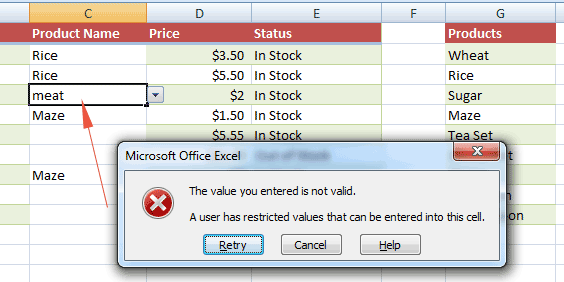
In the above example, an error will be displayed if you try entering a value that does not exist in the drop-down.
For example, our drop-down does not contain “Meat”. As I entered the value in a cell with a drop-down, this is how it displayed the error:
So, what if I want to allow entering other values apart from the drop-down?
This is quite easy to implement. Follow these simple steps to enable this.
After selecting the drop-down cells, go to the “Data” in the ribbon and locate the “Data Validation” group.
There, click on the “Data Validation” option as we did in the above example.
In the pop-up window, click the “Error Alert” tab as shown below:
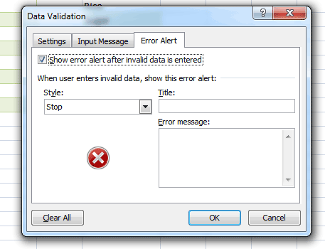
The option “Show error alert after invalid data is entered” should be pre-selected. Uncheck this option and press OK.
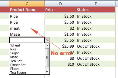
Now, Excel should not display the error message for entering other values than drop-down list.
Displaying a custom error message example
If you want users to enter only a value from the list and if some other value is entered, you want to show a custom error message. This is how you may do it.
After selecting the drop-down cells, go to the “Data” in the ribbon, and under the “Data Validation” group, click the “Data Validation” option.
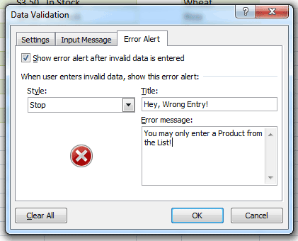
In the popup window, click the “Error Alert” tab and there you may enter the custom message as shown below:
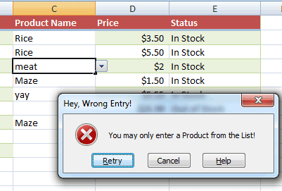
If a value other than the drop-down list is entered, this is how the custom message will display:
Using a data source other than cells example
Rather than selecting a range of cells as the source of values for the drop-down list, you may also enter the values directly in the source text box.
In that case, write the values in the source text box and just separate them by a comma as shown below:
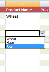
Now our drop-down list should show only three values entered in the source text box as shown below:
How to add new items in the drop-down example
After creating a drop-down list, you may be required to add, update, or remove the existing items in the drop-down.
For adding the new items based on the cells as the data source, simply insert a new cell at the desired position where you want that item to appear in the list and enter the value.
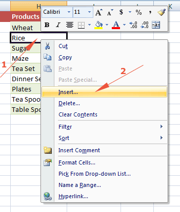
For example, in our list of the above demos, we don’t have “Meat” in the drop-down list. Suppose, we want to add this item.
Right-click on the cell that acted as the source of values for the drop-down list. I want to add the “Meat” after the Wheat, so I right-clicked on the “Rice” as shown below and clicked the “Insert” option:
Press the “Shift cells down” in the next window which should result in a blank cell under the “Wheat” item.
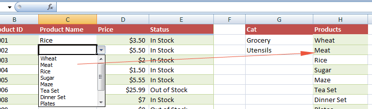
There I added the new item “Meat”:
You can see below the drop-down is also showing this new entry:
Removing an existing item
For deleting an existing item from the drop-down list based on cells, simply right-click on the item and click on the “Delete” option under the “Insert”.
Click on the “Shift cells up” in the next window and press “OK”. This should delete the existing item in the list.