Excel VLOOKUP Function
the VLOOKUP in Excel is used to “look up” or find a value in a table. The V in VLOOKUP function stands for Vertical. That means the VLOOKUP function works for data organized vertically.
What is Excel VLOOKUP function?
- Excel VLOOKUP is a function for finding and retrieving specific data in large tables.
- VLOOKUP works vertically and is case-insensitive.
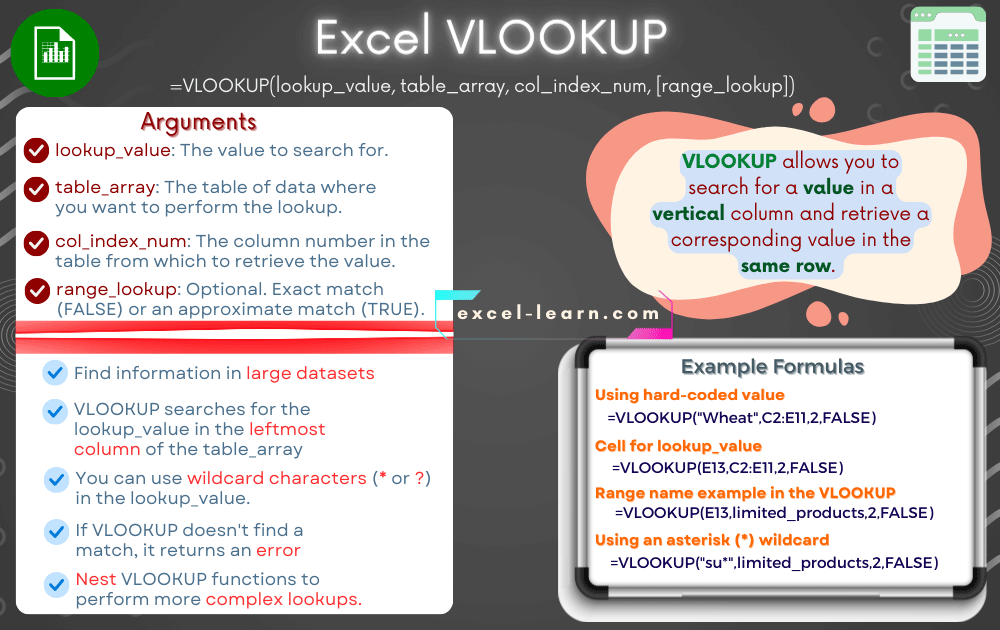
- VLOOKUP has arguments: lookup_value, table_array, column number, and range_lookup for exact or approximate matches.
- The function's versatility makes it a valuable tool for Excel users.
- 1. An Introduction to the VLOOKUP Function
- 2. The VLOOKUP example for getting the price
- 3. The example of using cell for lookup_name
- 4. How to do VLOOKUP if a table contains duplicate entries?
- 5. An example of range_lookup as TRUE
- 6. Using a range name example in the VLOOKUP function
- 7. An example of using an asterisk (*) wildcard in the VLOOKUP function
An Introduction to the VLOOKUP Function
Let me start with an example to explain what is Excel VLOOKUP function. If you know a little about VLOOKUP then move to the examples section below.
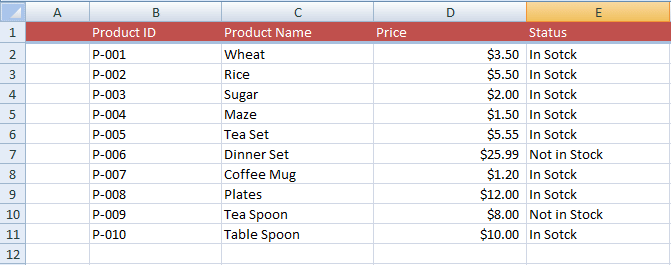
Suppose, you have a large Excel table that stores product information in a departmental store. The information includes Product ID, Product Name, Price, Status, Category, etc.
The table contains hundreds of records. Now, you want to find out the status or price of the Wheat bag quickly; how can you do that?
One of the ways is to “LOOK UP” the table information one by one and scan through your eyes (hope, you will find it soon without a headache) or use the VLOOKUP function – provide the known information like Product Name or ID and you are done. For example:
On that basis, let me define the VLOOKUP function:
| Argument/Point | Description |
| vertical column | As the name suggests, the VLOOKUP in Excel is used to “look up” or find a value in a "vertical" column. |
| lookup_value | The “Wheat” is called lookup_value. You may use the text, number, cell reference, etc as lookup_value.
The lookup_value must be in the first column of the table-array. In that case, Wheat must exist in the first column. |
| table-array |
|
| col_index_num | The 4 in the above formula tells the column number where we are looking for returned information, the price in that case.
So, the first column contains Product Names and 4th column contains the respective prices. |
| range_lookup | We used “FALSE” as the last parameter that specifies finding the exact match in the first column.
If the first column contains “Wheat” then it will return the price. If it contains “Wheat bags” then there will be no match. If you want to find out the closest match then use the TRUE value. The TRUE is the default. |
| "V" in VLOOKUP | The "V" in the VLOOKUP function stands for Vertical. That means the VLOOKUP function works for data organized vertically. Each row represents a new record. |
| Case insensitive | VLOOKUP is case insensitive. That means “Wheat” and “wheat” are treated the same way. |
Now let us look at a few examples in this tutorial based on the Products table for using the Excel VLOOKUP function to make things clearer.
The VLOOKUP example for getting the price
In this example, we will use the Product Name for the lookup_value and the function will return the corresponding price for that product.
The Excel table contains the following data where we will use VLOOKUP formulas:
The VLOOKUP formula for getting the price of “Wheat”:
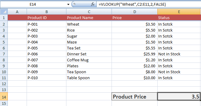
You can see, we used the “Wheat” to look up the Product Name column. As such, the Product Name belongs to the C column while product names start from C2, so our range started from C2 to E11 in the VLOOKUP formula.
The price belongs to the D column whose number is 2 in our specified range or table_array. So, VLOOKUP searched the Wheat in the left column and returned the price from the second column.
The example of using cell for lookup_name
In real scenarios, you may require entering any product name and the VLOOKUP function should return the price of that product. Unlike the above example where we used constant literal “Wheat” in VLOOKUP formula.
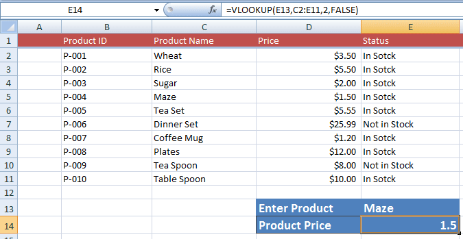
In this example, you may enter any product name; press enter and the price of the matched product will display in the specified cell. First, have a look and I will explain a little bit about how it is done:
VLOOKUP formula for any product:
The result as I entered Maze:
If you are running this example on your system after downloading the Excel sheet then follow these steps:
- Select the E14 cell and paste the above formula in the “Formula bar”.
- Enter any Product Name from the existing names in E13 cell and press enter.
- As we specified E13 in the VLOOKUP formula for “lookup_name”, the VLOOKUP function will take that name, find the price and display it in the specified cell (E14).
- Repeat the processes by entering other product names and checking how it updates the designated price cell.
How to do VLOOKUP if a table contains duplicate entries?
If your range contains duplicate entries for the “lookup_name” then the VLOOKUP function returns the first matched value.
To demonstrate that, I made a few changes in the example table. The product “Rice” is entered twice; one with “In Stock” and the other with “Out of Stock” values in the Status column. See the result yourself after using this VLOOKUP formula:
The output:
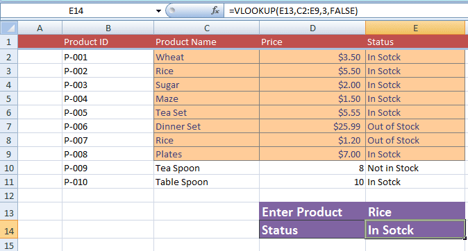
You see, even the second occurrence of Rice is “Out of Stock”, the Excel VLOOKUP function returned the first result only. The highlighted data in orange reflects the “table-array” in this example.
An example of range_lookup as TRUE
Until now, we explicitly used the FALSE value for the range_lookup (the last parameter in VLOOKUP).
- The FALSE value means an exact match as finding the lookup_value.
- Generally, you will use VLOOKUP function in that way. However, in certain situations, you may require finding the approximate match.
- For a close match, you may use the TRUE value. This is also the default value of the VLOOKUP function. So, if you omit this parameter, the VLOOKUP will find a close match.
- Using the TRUE value assumes the first column is sorted alphabetically or numerically and then it will search for the closest value. If not sorted, this may result in unexpected results.
See the following example where I just entered “p-1” and see if it displays the value for the closest match.
The result in Excel sheet:
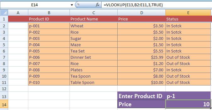
You can see that the Product ID is already sorted and it returned the p-010 price.
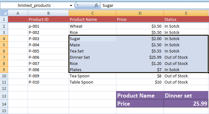
Using a range name example in the VLOOKUP function
In all the above examples, we used the range of cells by specifying cell numbers. You may also use range names using the VLOOKUP function. This may be particularly useful if you want to distinguish certain sections of the table from others.
Have a look at this example where I used a subset of data from our Products table (C4 to E9). For that, I created a range named, limited_products and used this in the VLOOKUP function as follows:
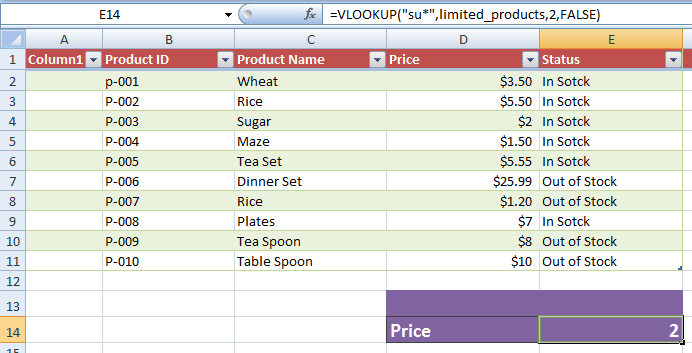
An example of using an asterisk (*) wildcard in the VLOOKUP function
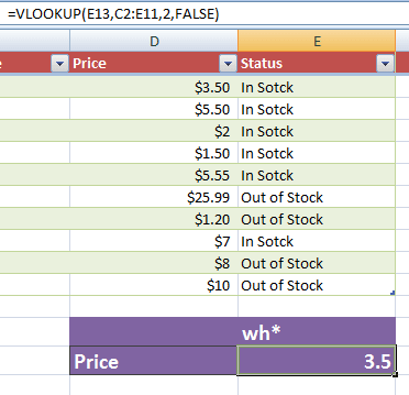
The * wildcard can be used if you do not know the “lookup_value” exactly. The '*' is used to match any sequence of characters. So, if we just enter the “su*” in our example sheet for VLOOKUP formula, see the outcome:
The result:
Similarly, you may use the question mark (?) wildcard that matches any single character. For example:
returns the same result as in the above example. However, you must provide the exact number of unknown characters as the question mark. This would have resulted in “N/A” with two question marks:
So, if our formula of VLOOKUP is this:
Enter the “su*” in E13 column will produce the same result: