5 Examples to Use Conditional Formatting in Excel [Highlight Cells Rules]

What is Conditional formatting?

Conditional formatting in Excel is the way to stand out or make different specific cells/information to others.

For example, making cell red for numbers less than a certain value.

Similarly, showing Out of Stock products as red to make them prominent over all products in the store.

Doing conditional formatting is easy in Excel and we will show you by different examples in the tutorial, so keep reading.

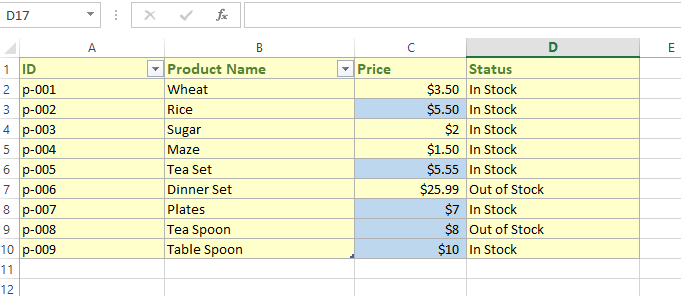
An example of making cells red with “Out of Stock” value

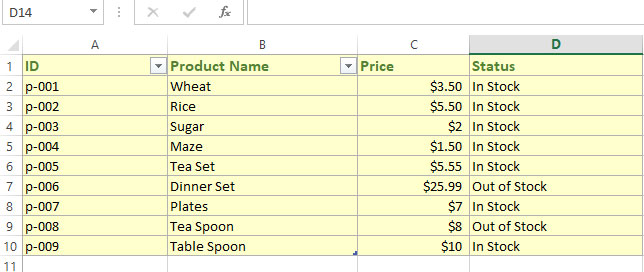
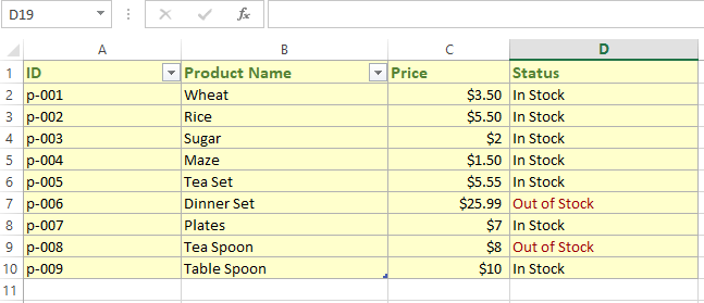
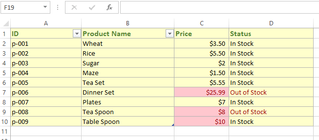
Let us start with a simple example of applying conditional formatting. Our target is making the D column (Status) red for which text is “Out of Stock”. The sample sheet is:

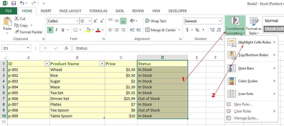
Step 1:

Highlight D column or Cells that you want to apply conditional formatting:

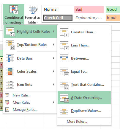
Step 2

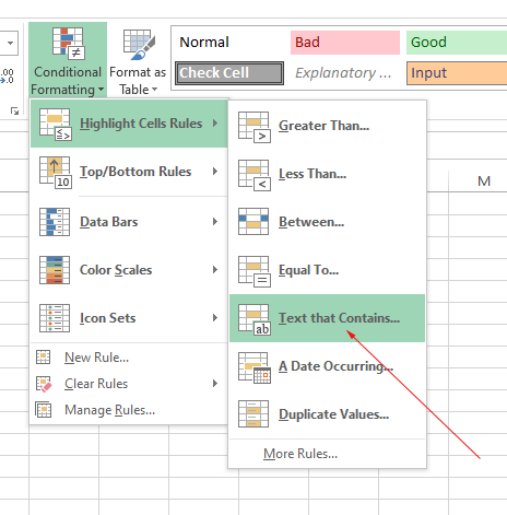
In the Home tab, locate “Conditional Formatting”. After clicking “Conditional Formatting”, click on the “Highlight Cells Rules”

Step 3

Click on the “Text that Contains…” option in the menu

Step 4

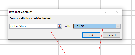
In the dialog box, enter the text that you want to make red. We wrote “Out of Stock” and select an option form “with” dropdown. We selected “Red text”. Click Ok.

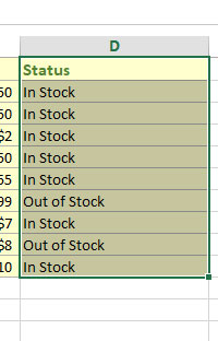
Result:

An example of using the Greater than option

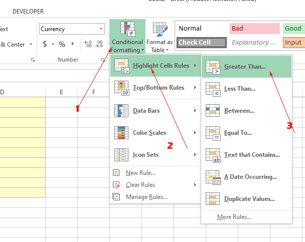
We will use “Greater Than” option under “Highlight Cells Rules” menu for this example.

Step 1:

Select the Price column

Step 2:

Click on “Greater Than”

Step 2:

In the “Greater Than” dialog box, write 7.00, and “with” select box, choose the “Light Red Fill with Dark Red Text” option.

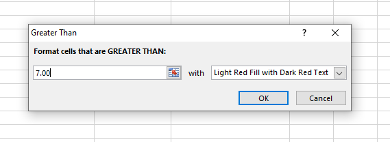
Result:

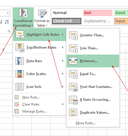
An example of Between option

Similarly, you may format cells that fall between two given values.

We will highlight the price column with values between five and fifteen inclusive.

Step 1:

Choose the Between option in “Highlight Cells Rules”

Step 2

In the “Between” dialog, enter 5 and 15 as shown below:

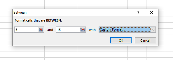
Select a formatting option as well. We chose “custom Format” option and set the style there.

Result:

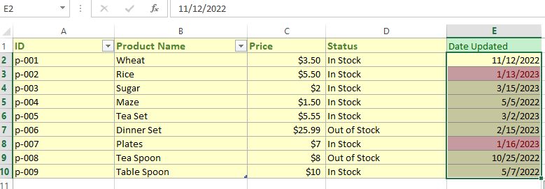
Formatting date column example

For this example, we have added a date column in the sheet with the dummy dates (for demo only).

Step 1:

Select the date column’s cells

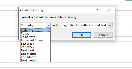
Step 2:

Go to Conditional Formatting --> Highlight Cells Rules --> A Date occurring

Step 3:

Select the date occurring option from the dialog and formatting option

Result as we selected “Last Month”:

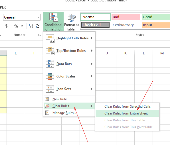
How to remove formatting?

In order to remove whole or selected cells formatting, again go to the “Conditional Formatting” and choose the appropriate option as shown below:

Further Learning for conditional formatting

To learn how to find duplicate data and remove it by using condition formatting, you may go to its tutorial.

Find and Remove duplicates in Excel