What is the purpose of IFERROR function?

The IFERROR function enables us to trap and handle the errors that occur in Excel functions or use independently.

You may display descriptive messages e.g. “0 is not allowed” etc.

This is natural that an error occurs as you run different Excel Formulas.

For example, #DIV/0! error occurs as you try dividing a number by 0.

Similarly, as VLOOKUP function is used to return a value for searched text and it does not exist. In that case, a #N/A (Not Available) error occurs.

Syntax for using IFERROR excel function

IFERROR(value, value_if_error)

• The value is the required parameter. It specifies the value to be checked for error.
• The value_if_error is also required. This is where you may use descriptive text to display as an error occurs in a function. If an error occurs, the IFERROR returns this value.

An example of handling divide by zero error

Let me start with a simple example of using the IFERROR function in Excel. For that, column A is divided by column B and the results are displayed in columns C. See the formula and example sheet below:

=IFERROR(A2/B2,"Cannot divide by Zero")

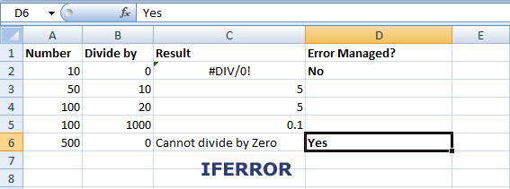
In the excel sheet, you can see C2 cell displayed the "#DIV/0!" error. This is because we did not use IFERROR there. The C2 formula is:

=A2/B2

So, it tried dividing 10/0 and an error occurred.

On the other hand, C6 displayed a descriptive message with no error. The formula for C6:

=IFERROR(A2/B2,"Cannot divide by Zero")

i.e. 500/0

It also generated the same error as in the case of C2, however, it is managed by using IFERROR.

An example of using IFERROR/VLOOKUP

In the above example, we used IFERROR independently. You may also use functions as the “value” argument in IFERROR. In this example, I will use the VLOOKUP Excel function with IFERROR. As such, the VLOOKUP is used to find a value in the given range or table-array. If the value is not found, #N/A error occurs.

To handle that, I have used VLOOKUP with IFERROR as shown below.

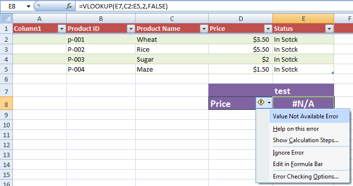
The VLOOKUP formula that produces an error without IFERROR:

=VLOOKUP(E7,C2:E5,2,FALSE)

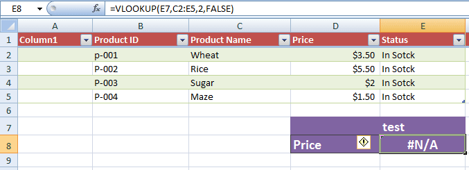
You can see, #N/A error is displayed on the E8 cell as I entered “test” in the E7 cell. If you look at the data, the Product Name column (C) does not contain the “test” value.

Now, entering the same “test” with IFERROR/VLOOKUP, see how it displayed descriptive information:

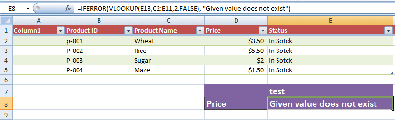
The formula:

=IFERROR(VLOOKUP(E13,C2:E11,2,FALSE), "Given value does not exist")

It makes more sense for future use if your excel sheet contains plenty of data and by mistake or unknowingly you enter the wrong information.

List of errors evaluated by IFERROR function

Following are the errors that can be evaluated and handled by using the IFERROR Excel function:

• #DIV/0!
• #N/A
• #REF!
• #VALUE!
• #NULL
• #NAME?
• #NUM!

An example of #VALUE error

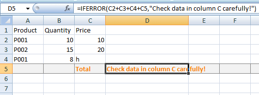
The value error may be raised for different reasons. For example, you are trying to add values of C2 to C5 cells and C4 or some other cell contains a non-numeric value. See the graphic below:

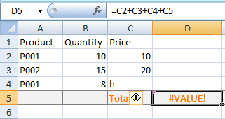
Now, I will use the IFERROR function to manage #VALUE! Error as follows:

=IFERROR(C2+C3+C4+C5,"Check data in column C carefully!")

The output as a non-numeric value is entered in C column:

It is looking better, isn't it?

Resolving the #NAME? error

The #NAME error occurs if a formula is entered incorrectly. For example, I entered the VLOOKUPs  as shown below:

Formula:

=VLOOKUPs(E13,C2:E11,2,FALSE)

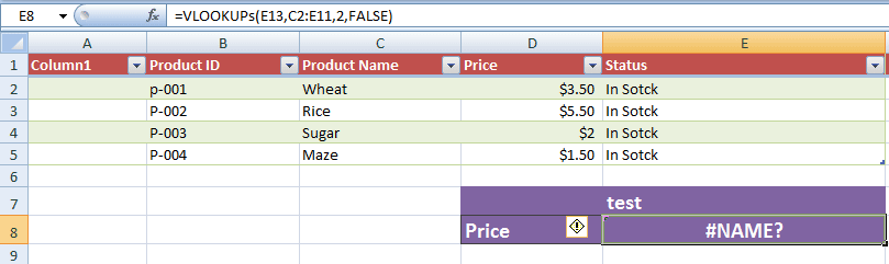
Although, you may use the IFERROR function to show a descriptive message. However, you should resolve it by looking at and correcting the formula name rather than using the IFERROR function.