A brief about line graphs

The line graph (also called line chart) is used to display the data graphically with lines that change over the period of time.

The markers or data points in line chart are connected by the straight lines. Generally, the line charts are used for visualizing the trends over the intervals like year on year, or month on month etc.

In this tutorial, I will show you step by step creating the line charts/graphs in Excel.

Creating line graphs in Excel

If you have data organized in the correct way then it is the matter of a few clicks for creating the Line graph in Excel. To demonstrate that, I will use dummy data of students. An Excel sheet is created that keeps records of the number of students getting specific grades every year.

So, a row contains a Year and number of student who got A+ Grade, A Grade, and B Grade. See the demo table below that will be converted into line graph:

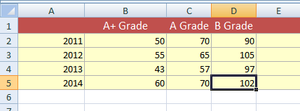
For simplification, I just created a few rows of data.

Follow these steps for creating this data into a line chart.

Step 1:

Select the cells that you want line chart display the information. In our example case, I selected A1 to D5 cells. Notice in the graphic below that no header is given for the year.

Step 2:

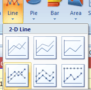
In the Ribbon, go to Insert --> Line as shown below.

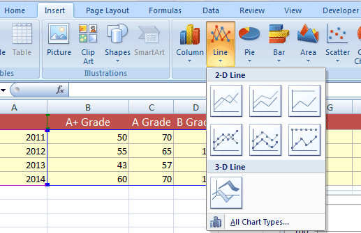
Select from the 2D or 3D Line options. For the demo, I used “Line” option in the top left. It allows creating the line graph that displays trends over time (dates, year etc.)

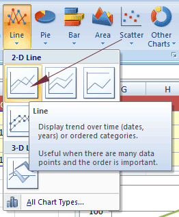
This option of Line chart is useful when there are many data points and order is important.

As you select an option, the graph should be created in Excel sheet based on selected cells data.

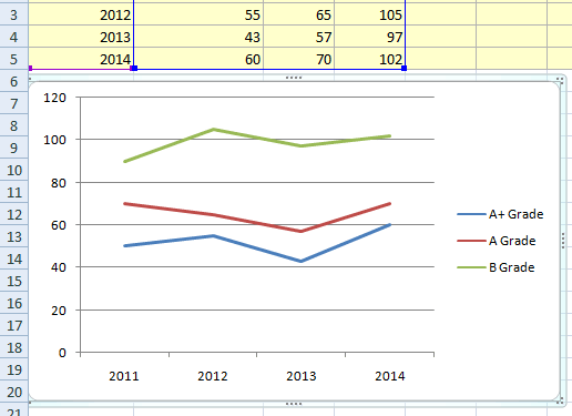
You can see, years are displayed on the horizontal side (x-axis) while the number of students with grades in the y axis.

Is not that pretty simple?

Now let us look at a few options for customizing the Excel line graph as per the desire.

Selecting the chart style

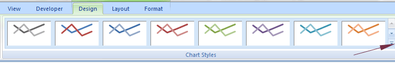
Excel has a number of built-in line chart styles that you may access via:

Go to Design tab; it is visible as you select the existing chart. In the chart style groups, you may select a style. To see the complete available styles, expand by clicking the right arrow as shown in the graphic below (red arrow):

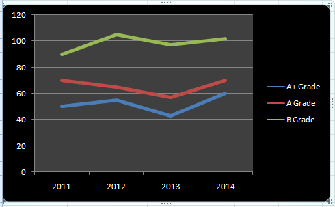
An example of a different chart style is displayed below:

Adding title in Line Graph

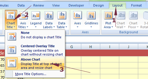
Having a title for the live graph for describing its purpose is important. For adding a title in the line graph, go to the “Layout” tab in the Ribbon.

In the “Labels” group, Click “Chart Title”. For adding a title above the line graph, click “Above Chart” as shown below:

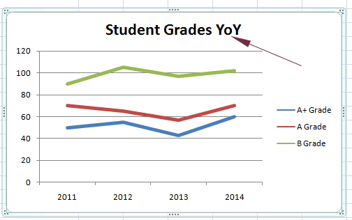
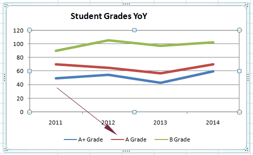
I entered the “Student Grades YoY” (year on year) for our example line graph.

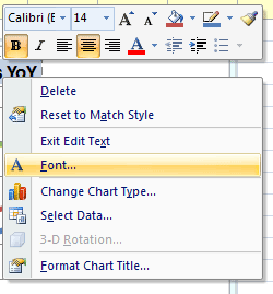
You may adjust the size, character spacing, Effects of title etc by right-clicking the title (after selecting title text) and press the font option:

How to Show Legends on top

In our examples, the legends (A+ Grade, A Grade, B Grade) are displayed towards the right side. You may want to display the legends towards the top, bottom, left etc.

For doing that, go to the “Layout” tab in Ribbon after selecting the graph. Find and press the “Legend” in the “Labels” group.

There, you may select the direction of legends in the line chart as shown below:

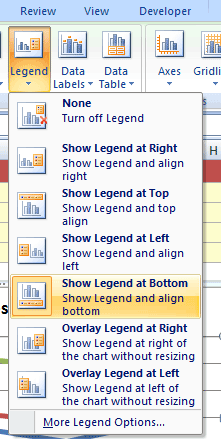
I selected “Show Legend at Bottom” and see how it displayed the line chart :

Try other options till the one fits best per your need.

Creating an Excel Line graph with Markers

In all above examples, we used the simple Line graph. Let me show you another available line chart with markers.

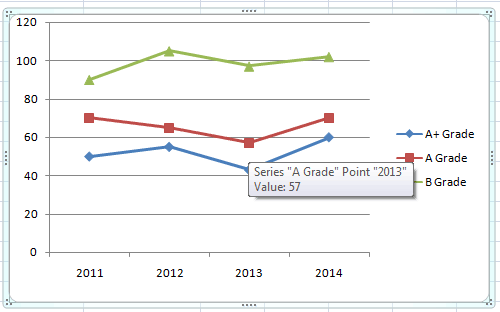
The line charts with markers are useful when you have a few data points. On mouse hover, the screen tip is also displayed with related information.

For creating a line chart with markers, follow these steps.

After selecting the cells, go to the Insert --> Line --> Line with Markers

A line graph with markets should have been created in the Excel sheet for the selected cells data:

How to update data in the previously created line chart?

There will be chances that you have created a line chart with lots of effort and in future, you may need to update it with new data. For example, in our Excel table (used for above demos), the student's data should be updated for coming years.

Until now, I showed examples with years 2011 to 2014. If we need to add the records of 2015 and 2016 and update in the line chart as well, how can we do that without recreating from the start?

One of the ways of updating the line chart is as follows:

Step 1:

Right click on the graph area where lines are displayed:

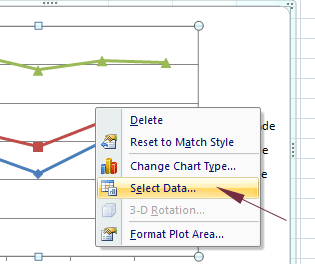
Click on the “Select Data” option. The Select Data Source dialog box should open as shown below:

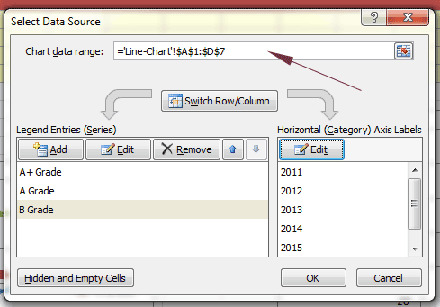
In the chart data range, you may see the range is specified. There, update the cell(s) that you want to include. For the example, I added two more records for 2015 and 2016 that goes till D7 cell. So I update the record from:

='Line-Chart'!$A$1:$D$5

To

='Line-Chart'!$A$1:$D$7

And see the graph now:

You can see, two more rows added and these are reflected in the line chart as well.