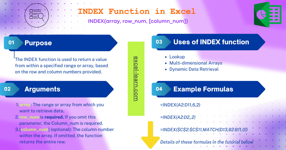
INDEX Function in Excel
The Excel INDEX function requires the position and range and returns the value based on that position. If you do not know the position, you may get this by using MATCH function.
- If you require finding the value in the specified range or array then use the INDEX function.
- The Excel INDEX function requires the position and range and returns the value based on that position.
- If you do not know the position, you may get it by using the MATCH function. So, you might hear a lot about the INDEX/MATCH combination.
- I will show you both in action in the coming section.
- 1. Syntax of INDEX function
- 2. The Excel INDEX for returning value example
- 3. The INDEX example with column_num argument
- 4. The example of using row_num and column_num arguments
- 5. Using INDEX and MATCH functions together
- 6. An example of using INDEX with reference
- 7. An example of getting SUM by using INDEX function
Syntax of INDEX function
The INDEX function has two variations.
First to return the value:
INDEX(array, row_num, [column_num])
Second, to return the reference:
INDEX(reference, row_num, [column_num], [area_num])
Let us first explore and see the examples of returning value by using the INDEX function.
The Excel INDEX for returning value example
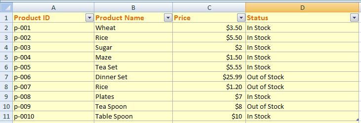
For our examples, we have the following style sheet that contains Product ID, Product Name, Price, and Status columns:
By using the INDEX function, we will find the value in B2:B11 range and within that range for row number 3. The INDEX formula:
=INDEX(B2:B11,3)
See the result as I entered this formula in D14 cell:
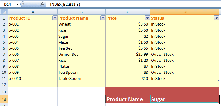
You can see that it returned Sugar. On that basis, let me explain the arguments in the INDEX function for returning value.
| INDEX Arguments | Description |
| array/range | The B2:B11 defines the range of cells. You may also use an array constant there. This is the range where we want to find a value as using the INDEX function. The array/range of cells is the required parameter. |
| If the array/range of cells contains only one row or column then the corresponding row_num or column_num is optional. | |
| row_num | The row_num is required. In our example, the 3 is the row_num that corresponds to the given cell range B2:B11. In that case, the third row contains Sugar that INDEX function returned. If you omit this parameter, the Column_num is required. |
| column_num | The column_num is an optional argument. If you omit this, the row_num is required (as in our example case). The column_num selects the column in specified array/range cells, from which to return value. |
See an example below where row_num is omitted and row_column value is provided to make things clearer.
The INDEX example with column_num argument
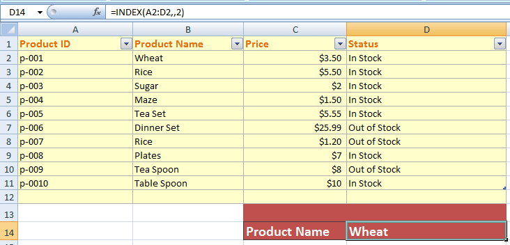
See the formula and resultant sheet as I provided the column_num argument as 2 while row_num is omitted.
The formula:
=INDEX(A2:D2,,2)
You may notice from above two examples, if column_num is omitted (in the first example), you have to use same column (e.g. B2:B11) in the INDEX formula for the range of cells.
If you omit the row_num argument, then range of cell must be from the same row (e.g. A2:D2). If we used A2:D4 in above example, an error would have produced.
The example of using row_num and column_num arguments
Now let me use both arguments in the INDEX function and show you the result and conclude how it worked. First, have a look at this formula:
=INDEX(A2:D11,6,2)
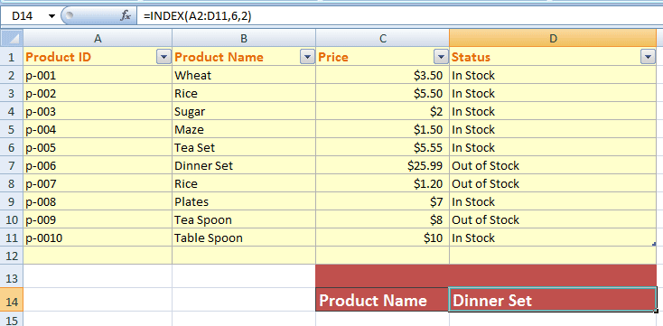
You can see, the row number 6 and column number 2 contains the “Dinner Set” product name. If you count the given range, the first column is Product ID and second is Product Name that we specified as the column_num. While row number 6 and column 2 intersection contains Dinner set.
Using INDEX and MATCH functions together
When you have large data tables in Excel and you need to find the values based on position then you may use the INDEX in conjunction with MATCH function.
The MATCH function returns the position of the specified item for the given range or array. The MATCH returned value may act as the row_num or column_num argument for the INDEX function.
Consider the following scenario based on our example sheet. Suppose, we only know the product names (e.g. Wheat, Sugar, Maze) that are stored in the excel sheet. On that basis, we need to know the price of a product along with its status (in Stock or out of stock).
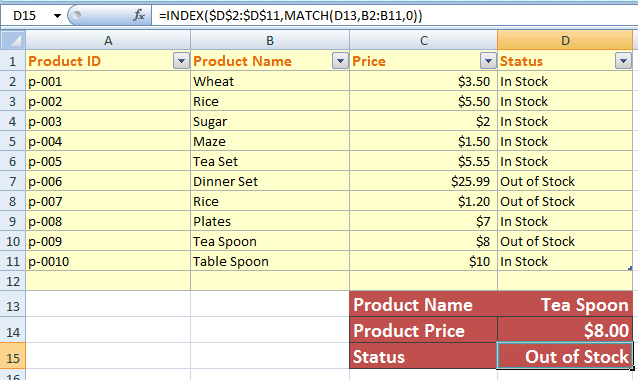
See the following formula of INDEX/MATCH and example sheet that enables us fulfilling these two requirements:
For retrieving the price:
=INDEX($C$2:$C$11,MATCH(D13,B2:B11,0))
For retrieving status:
=INDEX($D$2:$D$11,MATCH(D13,B2:B11,0))
The result for different products:
Tea Spoon:
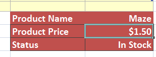
For Maze:
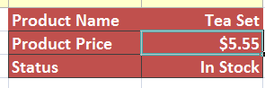
Tea Set:
You may also use the wildcards in the MATCH function. For example, I just entered “R*” and see what it returned:
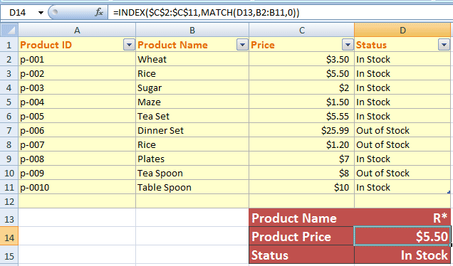
In the Excel sheet, you can see that Rice occurs twice. One is B3 cell and the other is B7. The MATCH function returned the position of the first occurrence. So, if you have duplicate records and using the MATCH function, it only returns the first match.
Similarly, you may use the ‘?’ wildcard:
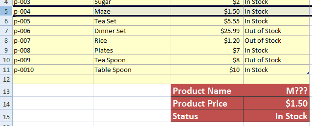
The Product name entered in D13 as “M???” and it returned the record of Maze.
An example of using INDEX with reference
As mentioned earlier, the INDEX function has two variations; one returns value and the other returns reference of the cell at the intersection of particular row and column.
The syntax is:
INDEX(reference, row_num, [column_num], [area_num])
See an example of using two ranges in the INDEX function and I will explain the arguments after that:
The formula with two ranges:
=INDEX((A1:C6, A8:C11), 2, 2, 1)
The result of the above formula is:
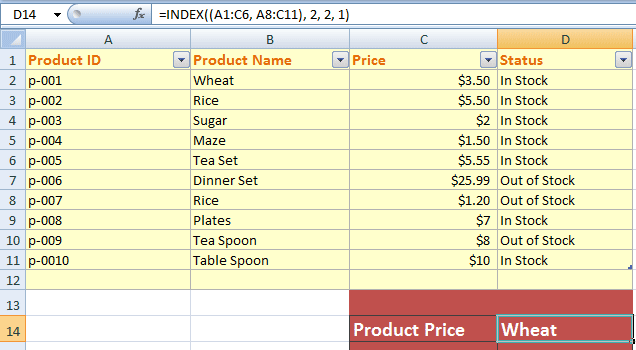
So why it return Wheat as I entered that formula in the D14 cell? Let us go through the arguments and you will understand that:
The INDEX function arguments (reference)
| INDEX Arguments | Description |
| Reference | Reference is required. This is the reference to one or more cell ranges. I used A1:C6 and A8:C11 ranges.
You may also use non-adjacent cell ranges as used in the above example. |
| Row_num | Row_num is the required argument.
This specifies the number of rows in the reference. I used 2 in the example. |
| Row_column | Row_column is optional.
This is the number of columns in the reference. This is where the INDEX function returns the value. I used 2 value for this in the formula. |
| Area_num | Area_num: The last and optional argument.
This argument selects the range in reference (remember I gave two ranges in the formula). If you do not use this argument, the 1 value is used by INDEX. The first area is selected or entered is number 1, and after that number 2, and so on. I used 1 value in the formula – so it used the A1:C6 range. In the A1:C6 range, the second column is Product Name while the second row contains Wheat; thus INDEX returned Wheat. |
The A8:C11 in our example formula is the Area_num 2. If we give 2 for Area_num in the same formula then see the result:
The formula and result:
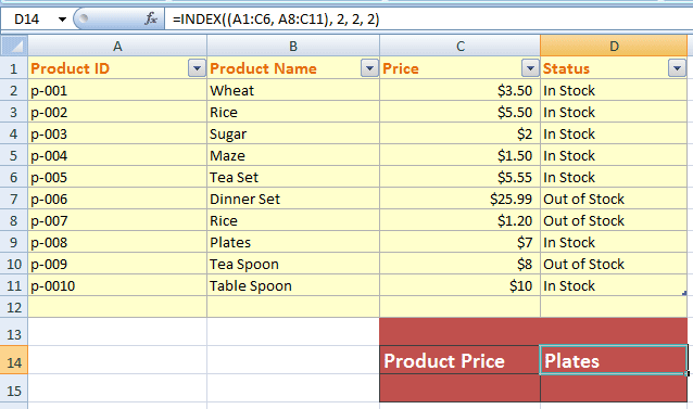
You can, I used the same argument value; two ranges (A1:C6, A8:C11), 2 row_num, 2 column_num, and only changed area_num from 1 to 2.
The INDEX function used A8:C11 range and returned the “Plates”.
An example of getting SUM by using INDEX function
In this example, I will write the formula for getting the sum of the Product Price column in our example table by using the SUM with the INDEX function.
The formula of SUM/INDEX:
=SUM(INDEX(A2:C11,0, 3,1))
The result:
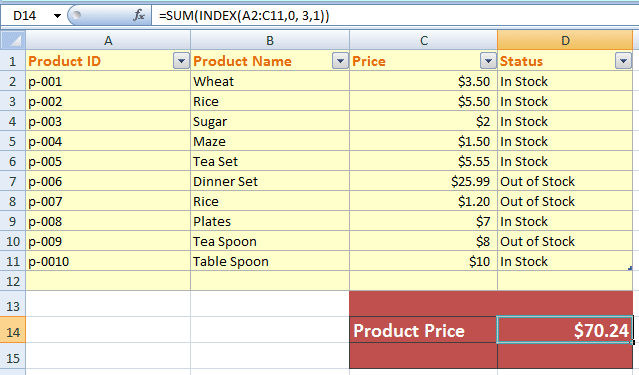
You can see, the area_num 1 (A2:C11) with column number 3 values used the C2 to C11 cells and returned the SUM of Product Price.