MATCH Function in Excel
The Excel MACTH function returns the relative position of the specified item from the given range of cells. This is how the MATCH function can be used:
The Excel MATCH function returns the relative position of the specified item from the given range of cells.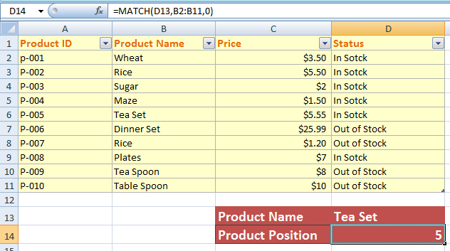
For example, we have fruit names in column B:
- Apple
- Mango
- Banana
- Strawberries
- Orange
We want to search the position of Banana; this is how the MATCH function can be used for that:
The return result will be 3. On the basis of this formula, let us explore the arguments of the MATCH function after its general syntax.
- 1. Syntax of the MATCH function
- 2. An example of MATCH in EXCEL
- 3. Using the cell reference in MATCH function
- 4. An example of searching in rows (horizontally) by MATCH function
- 5. Exploring the Match_type argument
- 6. Data contains duplicate values with 0 value
- 7. Using the 1 value for Match_Type example
- 8. Using the -1 for Match_Type
- 9. Using INDEX with MATCH function
Syntax of the MATCH function
In the syntax:
| Argument | Description |
| lookup_value |
|
| lookup_array |
|
| match_type |
|
An example of MATCH in EXCEL
The first example uses the Excel sheet that stores Product information like Product ID, Product Name, Price, and Status.
We will find out the relative position of a product; first by vertical lookup and in the next example horizontally.
The formula used for the MATCH function to search “Maze”:
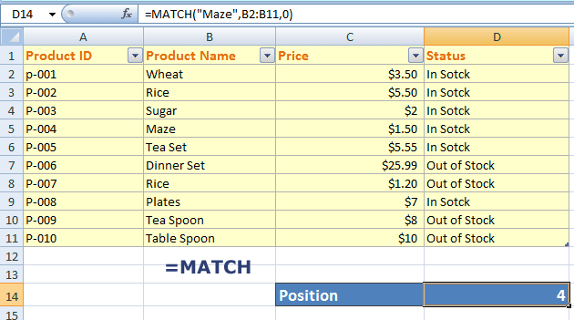
You see, in the given range (B2:B11), the position of Maze is 4.
Using the cell reference in MATCH function
It is not generally a good practice to use constant literals in formulas as used in the above example for the demo only. For the next example, I will refer a cell (D13) in the MATCH formula. Just enter the product name in D13, press enter and D14 will be updated by the product position in the given look_up array.
The following formula is used in D14 cell:
An example of searching in rows (horizontally) by MATCH function
You may also use the MATCH function for searching the product position of horizontally managed recordsets.
For that, refer to the range of the look_up array for the same row e.g. A2:E2. If you refer to something like this: A2:E5 then an incorrect result may be returned by the Excel Match function.
For demonstrating that, I will search the position of “Plates” in A9 to D9:
The formula:
As I entered the Product price = 7, see the result:
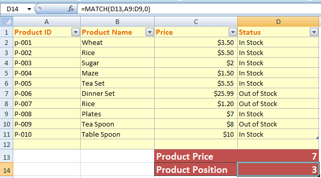
It returned position = 3.
Exploring the Match_type argument
The third argument in the MATCH function is Match_type. Until now we used zero value for all the examples in above section. Following are the details of three possible values:
| Value | Description |
|---|---|
| 1 | This is the default. If you omit this argument, the 1 is taken. It specifies finding the largest value that is less than or equal to the lookup_value. If you use this option, ensure that the values in lookup_array are in ascending order. |
| 0 | The 0 value means to find the exact match while lookup_array values are in any order. It finds the first matched position.
So, if your lookup_array has duplicate values, the first matched position is returned. |
| -1 | This value finds the smallest value which is greater than or equal to the lookup_value. In that case, the lookup_array values must be placed in descending order. |
Now let us have a look at a few examples in the Match_Type argument.
Data contains duplicate values with 0 value
In our example sheet, the product name “Rice” is entered twice. See the output as we search the Rice position by MATCH function with 0 value for Match_type:
The formula in D14 cell:
The result:
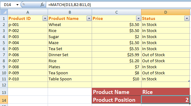
You can see that it returned the first matched position i.e. 2 rather than 7 (the second occurrence).
Using the 1 value for Match_Type example
For that, I have changed the Product ID column value to numeric format and placed it in ascending order. See the formula and output for different entries:
The MATCH formula in D13:
The results:
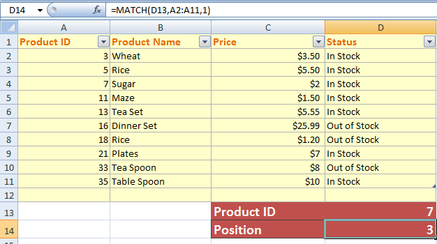
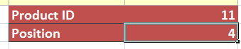
Entered 9:
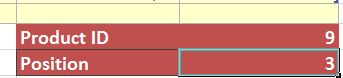
Entered 11:
You can see that even though the value 9 does not exist, it returned the closest match. If we use 0 value for Match_Type, the output is:
Formula:
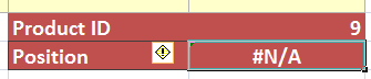
A #N/A error occurred.
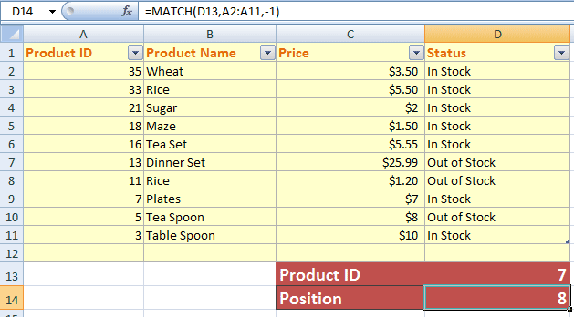
Using the -1 for Match_Type
First, have a look at the output if we used the same dataset as in the above example and used the -1 match_type:
The Formula:
The output for 7:
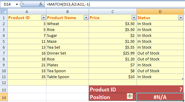
It produced a #N/A error when I entered 7. Though 7 exists, however, lookup_array is not sorted in descending order with -1 which resulted in an error.
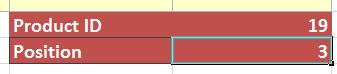
Now have a look at the output as I re-order the Product ID column in descending order and enter 7 and other values:
Output as 7 is entered:
For value 19 that does not exist:
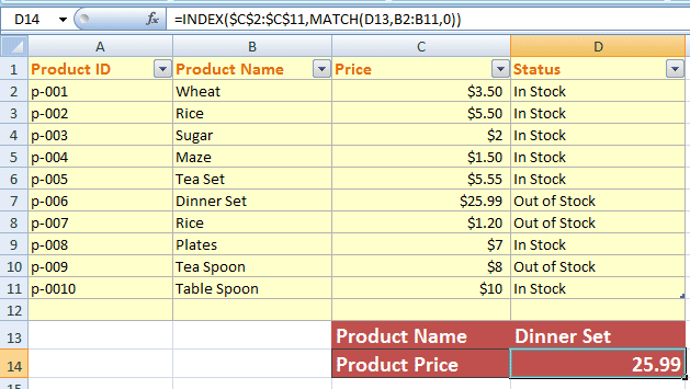
Using INDEX with MATCH function
The INDEX function is used to return the value from the given array, range, or table. The syntax of the INDEX function is:
You may provide the row_num or column_num value by using the MATCH function and the INDEX function will return its value.
See the following example for learning how to use the INDEX and MATCH functions together.
For that, I used the same spreadsheet as in the above examples. This time, I will enter the Product Name in the D13 cell, and the INDEX/MATCH combination will return the price from the C column for the entered product.
The Formula of INDEX MATCH:
The result for Dinner Set:
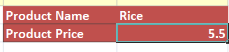
For Rice product name:
As mentioned earlier, you may use the wildcard characters (* and ?) if Match_type in MATCH is 0 and lookup_value is text. This perfectly suits the above table and the same formula. See the results:
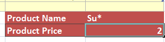
If you look at the complete graphic of table data then it returned the Sugar price.
Similarly, using the ‘?’ mark wildcard:
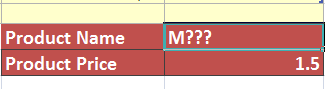
It returned the Maze price.