3 Examples to Learn Excel MOD Function to Get Remainder

What is Excel MOD Function

The MOD function returns the remainder after a number is divided by the divisor.

For example:

= MOD(12,3)

It will result in 0.

In this case:

The 12 is the number.
3 is the divisor.
0 is the remainder after 12 is divided by 3.

Syntax of using MOD function

The general syntax is:

= MOD(number, divisor)

Both arguments are required in MOD function.
The MOD function result has the same sign as the divisor. If the divisor is a negative number then the result will be negative.
A #DIV/0! Is returned if the divisor value is 0.
The result of the MOD function can be achieved by using the INT function. For example:

If we have a MOD function like this:

MOD(12, 3) = 0

The result by using the INT function will be the same for this:

= 12 - 3*INT(12/3) = 0

The section below shows a few examples of MOD function with Excel screenshots.

The MOD function is available in the following versions/platforms:

Excel for Office 365 Excel for Office 365 for Mac Excel 2019 Excel 2016 Excel 2019 for Mac Excel 2013 Excel 2010 Excel 2007 Excel 2016 for Mac Excel for Mac 2011 Excel Online Excel for iPad Excel for iPhone Excel for Android tablets Excel for Android phones Excel Mobile Excel Starter 2010

An example of MOD Excel function

In this example, the cells from A2 to A6 contain the numbers while B2 to B6 divisors.

The MOD formula is applied to cells C2 to C6 for respective A and B cells.

To explain how the MOD function produces the result, different values with mixed signs in A and B cells are given. See the results below:

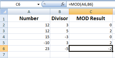
You can see, the result of the cells

=MOD(A2,B2) = 0

=MOD(A4,B4) = 0 (though we used -3)

=MOD(A6,B6) = -3 (as -5 value is used for B6)

Getting the sum of even numbers example

Generally, the MOD function is not used independently but with other complex formulas.

In the example below, we have numbers in A cells. The target is to get the sum of only even numbers in those cells.

For that, we can use the MOD function and check the number is each target cell. If the result of the division of that number by 2 is zero that means it is an even number.

Then, we used the SUMPRODUCT function to get the total of all even numbers as follows:

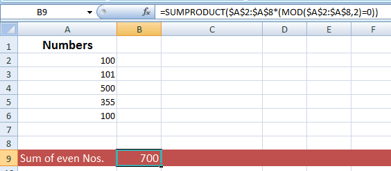
The formula:

=SUMPRODUCT($A$2:$A$8*(MOD($A$2:$A$8,2)=0))

Using the INT function as MOD replacement

For very large numbers, the MOD function may produce #NUM error.

As mentioned earlier, you may use the INT function as a replacement for the MOD function in that case.

The general way of expressing the INT as MOD function is:

= n – (INT (n/d) * d)

n= number
d = divisor

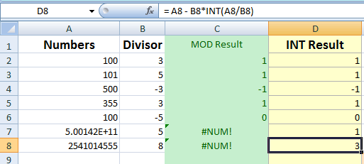
To show how INT works, I used the same Excel sheet as in the first example and added another column i.e. INT Result (D2 to D6 cells).

This is adjacent to the MOD Result and uses the following formula for corresponding A and B cells (in the case of A4 and B4):

= A4 - ( B4*INT(A4/B4))

See the numbers, divisors and result for both:

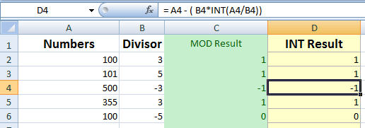
You can see, both MOD and INT functions produced the same results.

Also, see the sheet below where I added two large values and you can see the MOD function produced the #NUM! error while the INT function resulted in the remainder: