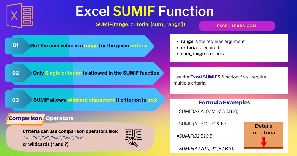
Excel SUMIF Function
If you require sum of a range with certain condition then use the SUMIF function. If you separate SUM + IF, it already makes you understand why we use that.
- If you require the sum of a range with a certain condition then use the SUMIF function.
- If you separate SUM + IF, it already makes you understand why we use that.
- For example, return the SUM of A2 to A10 cells IF the value is greater than 100.
- In that case, the SUMIF will return the total of all cells that contain numbers greater than 100.
An example of SUMIF and explaining its syntax
First, let me show you an example of using SUMIF with a single column that contains numbers. On that basis, we can understand its syntax easily.
In the example, the A2 to A10 cells are assigned numbers. We will get the sum of all cells whose numbers are greater than or equal to 100. The SUMIF formula:
=SUMIF(A2:A10,">=100")
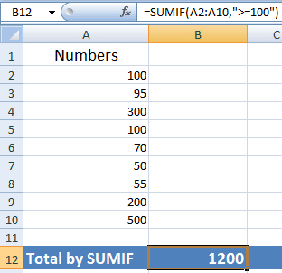
You can see, the SUMIF function omitted the numbers less than 100 and returned the sum.
Syntax of SUMIF function
The general syntax of using the SUMIF function is:
SUMIF(range, criteria, [sum_range])
We used only two required parameters in the above example, where:
| SUMIF Arguments | Description |
| range | A2:A10 is the range. This is where the criteria will be evaluated.
In our example, the value greater than or equal to is checked on A2 to A10 cells only. The SUMIF will ignore blank or text values in cells. You may also use dates in cells. |
| criteria | “>=100” is the criteria. You may use a number of criteria like “<100”, “>100”, “<>100”, “<=100”, “100”, B3, “text_string” etc. |
| sum_range | The third argument sum_range is optional. This is the actual range that is summed if provided.
If you omit this argument, the same range is used that defined criteria. In our example, we omitted this argument, so SUMIF returned the sum of the A2:A10 range. An example of using sum_range is given in the section below. |
The example of using sum_range in Excel SUMIF function
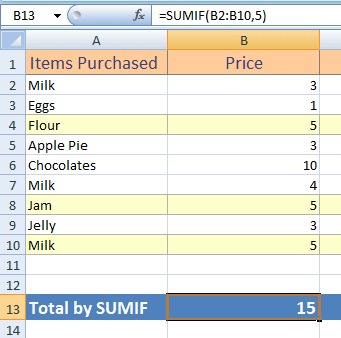
For this example, I will also use the sum_range argument. The SUMIF will actually get the total from this range, however, the range is filtered based on the given criteria. The formula of SUMIF:
=SUMIF(A2:A10,"Milk",B2:B10)
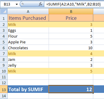
In the output, you can see three occurrences of “Milk” in A2:A10 cells. The SUMIF took the numbers from B2:B10 range and returned those three cell’s total. See the output if we used A2:A8 range:
=SUMIF(A2:A8,"Milk",B2:B10)
The result:
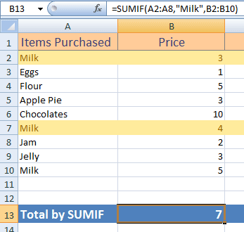
Now it only returned the sum of the first two occurrences of the “Milk”.
Using the cell reference in the criteria
The following example shows using the cell reference in the in the SUMIF criteria:
The formula of SUMIF:
=SUMIF(A2:B10,">" & B7)
The result:
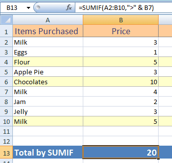
The SUMIF found "4" value in the B7 cell and so returned the total of three cells whose value is greater than 4.
Specifying a number for getting the SUM example
Rather than a condition, you may also use a simple number in the SUMIF function criteria to find the matches in the given range and return the total.
See an example below:
The formula used:
=SUMIF(B2:B10,5)
Using wildcards for text-based criteria example
The SUMIF function also allows the use of wildcard characters if a criterion is a text (as used in one of the above examples with “Milk”). In the following example, I used “J*” for criteria and see the result:
=SUMIF(A2:A10,"J*",B2:B10)
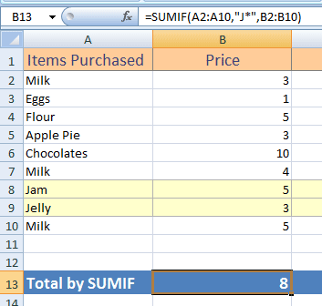
You can see, it summed up the Jam and Jelly prices and returned 8.
Similarly, you may use the ‘?’ question mark wildcard in the SUMIF function. The ‘?’ matches the single character while ‘*’ matches any sequence of characters.