The MROUND function for rounding nearest to 5, 10, 100, 1000 etc.

To get the nearest multiple for any number like 5, 10, 100 etc. you may use the MROUND function in Excel.

The MROUND function takes two arguments:

MROUND(number, multiple)

The number and desired multiple.

See the examples below for using the MROUND function.

The example of nearest multiple of 5

The nearest multiple of 5 means the closest number that can be multiplied by 5. For example:

• 8 Is closer to 10
• 11 is closer to 10
• 17 is closer to 15 rather 20
• 24 is closer to 25 rather 20 and so on.

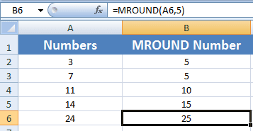
See the following example of getting the nearest multiple of 5 by using MROUND function. In the example, I used different numbers in the A column of excel sheet. The respective B cells display the nearest multiple of 5 where MROUND functions are used:

The formula for B2:

=MROUND(A2,5)

Getting the nearest multiple of 10 by Excel MROUND

In this example, the nearest multiple of 10 is displayed by using the MROUND function:

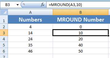
The formula used in A2 for nearest 10:

=MROUND(A2,10)

The example of getting nearest 100

Similarly, specify the value 100 as the second argument in the MROUND function for getting the nearest multiple of 100. See the MROUND formula and output below:

The formula for the nearest multiple of 100:

=MROUND(A3,100)

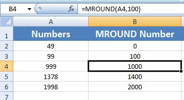
You can see, the nearest multiple of 99 is 100, 49 is 0, 1378 is 1400 etc.

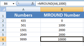
Nearest multiple of 1000 example by MROUND

See the following example for getting the nearest multiple of 1000 for the given numbers:

The nearest multiple of 1000 formula:

=MROUND(A3,1000)

In the same way, you may get the nearest multiple of any number like 0.5, 2, 3, 10000, 10000 and so on by using the MROUND function.

Getting the nearest multiple of 10 by ROUND function

You may also use the ROUND function of Excel to get the nearest multiples of 10, 100, 1000 etc. See the following examples of ROUND in action.

The first example shows how to get the nearest multiple of 10 by ROUND function.

The ROUND formula:

=ROUND(A2,-1)

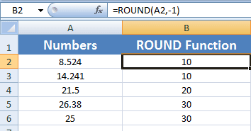
You can see, I used -1 value for the num_digits argument of ROUND function to get the nearest multiple of 10.

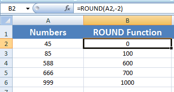
The example of nearest 100 by ROUND function

Similarly, use the -2 value for the num_digits argument for getting the nearest multiple of 100 for the given number.

The formula applied in B2 cell:

=ROUND(A2,-2)

For getting the nearest multiple of 1000, use the -3 value for num_digits argument.

You may learn more about the Round function in excel.