Hide/Unhide the Columns or Rows in Excel

How to hide a column in Excel?

To hide one column in Excel, follow these steps.

Select the column that you want to hide by clicking on the letter: A, B, C, etc. It should select the whole column as shown below:

Now, right-click on any cell of that column and click on the “Hide” option in the menu:

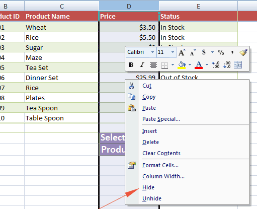
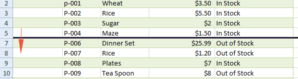
This should hide the selected column. For our demo, I selected the D column and clicked on the Hide option in the menu, after right clicking on a cell and see the result:

You can see, the D column is disappeared.

Hiding multiple columns by single click example

By following the above method, you may hide as many columns as you want; one by one. However, if you want to hide two or more columns that are not adjacent by a single click, follow this.

Suppose we want to hide the columns B and D.

Select the B column by clicking on the letter “B”.

Press the Ctrl key on the keyboard and select column “D”.

If you want to hide more columns then keep pressing the Ctrl key and select those columns.

This is how columns B and D look after we selected:

Right-click on any of the cells of column B or D and press the Hide option as shown in the first example.

Hiding a single-row example

This is how you may hide a single row.

Select a row by clicking on the row number. Suppose, we want to hide row number 6 in our demo sheet:

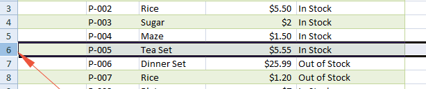
Right click on the row number or any cell of that row and click on the Hide option in the menu as we did to hide a column.

The result of this is hidden sixth row is as shown below:

Hiding multiple rows that are not adjacent

1. Just like hiding multiple columns that are not adjacent; for hiding multiple non-adjacent rows, select a row by clicking on the row number.
2. Press the Ctrl key and select the other row(s) that you want to hide.
3. Right click on any of the selected row numbers or their cells and press the “Hide” option. That’s it!

Unhide the hidden row or column

To unhide the hidden column or row, the procedure is simple and alike. Follow this to unhide the hidden row or column.

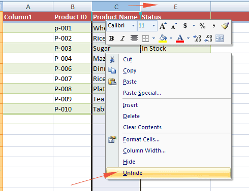
Select any of the adjacent columns of the hidden column. In our first example, we have hidden the D column. To unhide this,

Right click on the C or F column and click on the “Unhide” menu option as shown below:

Unhide by double line

If you look closer at the column lines after hiding a column, you will notice those are double lines and look a little thicker than normal columns. See the image below:

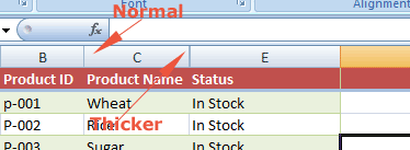
Similarly, the hidden row border is thicker which indicates the hidden row. You may double click or drag the lower line to unhide a row.

Hide/Unhide columns/rows in the ribbon

This is how you may hide the column, rows, and even the worksheet by using the main menu in the ribbon.

I will show you how to hide the column while the process of hiding the row remains the same as in the above examples.

Select the column you want to hide by clicking on the column head e.g. A, B, C, etc. I selected D column.

Go to the “Home” tab in the Ribbon.

Locate the “Cells” group and there you can see the “Format” button along with others as shown below:

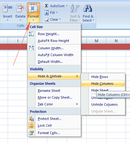
Under “Visibility” you can see “Hide & Unhide”. Open its menu and click on the “Hide Columns” option.

It will hide the selected column(s).

Similarly, you may hide or unhide the selected rows by using respective menu options.