How to Identify/Remove Duplicate Data in Excel sheet

• Finding duplicate data is quite simple in Excel.
• You do not require writing any formula but following a few mouse clicks in the menu/Toolbar.
• In this tutorial, I will show you step-by-step how to find duplicate data in rows/columns in different ways.
• This is followed by steps for deleting the duplicate data.

Step 1 – Find the duplicate data

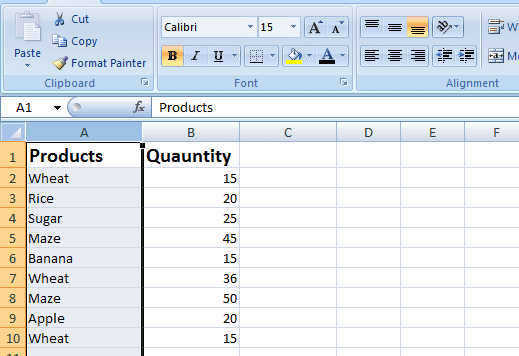
First of all, select the cells or range in your Excel sheet that you want to identify for duplicate data.

For demonstration, I have selected the A column only as shown below:

Step 2 – Locate the Conditional Formatting Button

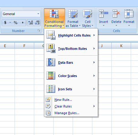
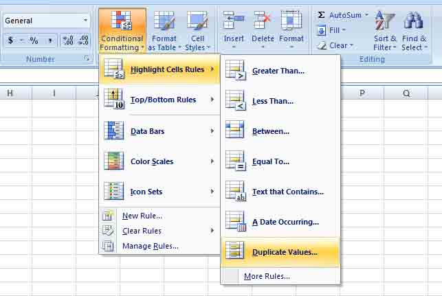
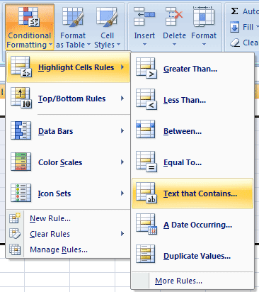
In the Home tab, find the Conditional Formatting as shown below:

Step 3 – Find Duplicate Values option

Go to Highlight Cells Rules --> Duplicate Values

Step 4 – finding the duplicates

After clicking the Duplicate Values menu option, a dialog box appears as shown in the following graphic:

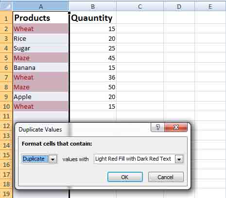
You will see that the duplicate values are highlighted as soon as “Duplicate Values” dialog appears.

In the dialog box, you can see “Format cells that contain” dropdown with two options: Duplicates and Unique. The Duplicate is the default value.

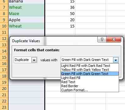
In the next dropdown, you may select the “value with” and select the formatting style that you want. Either use pre-defined or select the “Custom format” option for customizing the appearance of duplicate data.

You are done with identifying the duplicate data!

How to remove duplicate data in Excel Sheets?

Before exploring further for searching duplicate data in specific rows or columns and identifying duplicates with certain rules in this tutorial; let us have first a look at the steps of removing duplicate data.

Removing duplicate data is even simpler than searching it. Again, it is all based on a few clicks. Follow these steps:

Step1 – Selecting the data

Select the data that you want to find and remove duplicates. For the demo, I have selected columns A and B (Product and Quantity).

Step 2

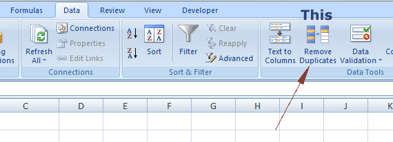
Go to the “Data” tab and find “Remove Duplicates” button:

The dialog for “Remove Duplicates” will appear. There, you may see and confirm which columns to remove data from. The  “My data has headers” checkbox will take the headings from columns.

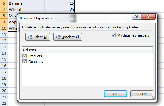
If you want to remove from all columns then press the “Select All button”.

I selected only “Product” column and see how many records were deleted:

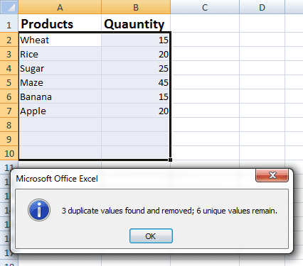
Removing duplicate rows

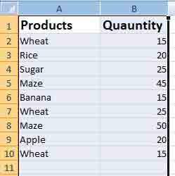
Excel removed all identical data except the first one in the above example. If I select all columns (Product and Quantity) then see the output before and after using Remove Duplicates tool:

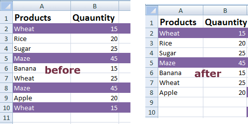
You can see that two duplicate rows are deleted from the Excel sheet.

For immediate recovery of data, you may undo the operation from the menu or press Ctrl+z key.

Highlight duplicates only for the specific value

Back to searching duplicates; in our first way of finding the duplicate values, we selected the cells, and all duplicate values were highlighted. What if you want to highlight the only specific value in the complete sheet for duplicate occurrence?

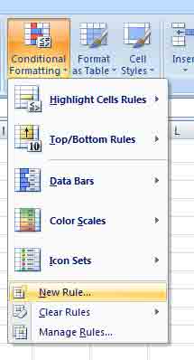
For that, you may use the “New Rule” under the “Conditional Formatting” option as follows.

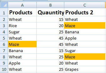
First, have a look at this example sheet:

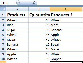
Now, we want to highlight only the duplicate occurrence of “Maze”.

Step 1:

Select the cells where you want to find and highlight the specific value. I selected from A1 to C10.

Step 2:

Again go to the Home à “Conditional Formatting” and select “New Rule”.

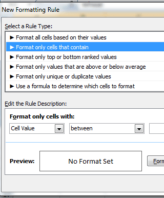
In the “New Rule Formatting” dialog box, select the “Format only cells that contain”

Under “Edit the Rule Description”, select specific text from the first dropdown with “containing” in the second dropdown and enter “Maze” text:

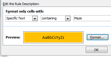
Use the format option for highlighting color as per your liking and press OK. See the result:

You can see, all Maze values are highlighted for the selected cells.

You may use the other options in the dropdown for specifying the numeric value with “equal to”, “greater than or equal to”, “between” for two numbers, etc. Similarly, if you have a date column, you may also select the “Dates occurring” option.

Another quick way of highlighting the filtered duplicate values

The second way of highlighting the specific duplicate cells based on a given text, numbers, dates, etc. is even simpler. For that, again go to the Conditional formatting under the Home and select “Highlight Cells Rules”.

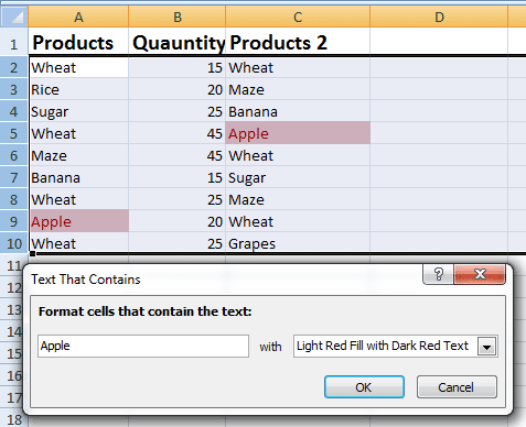
Unlike the first example in this tutorial for selecting the duplicate value, this time select “Text that contains” option.

Enter the text and formatting style and see how it highlights the duplicate values in the selected cells.

Note that, these tools are not specifically for duplicate checking (as we can see in the second last option “Duplicate Values”). You may also use the Between option for specifying two numbers and Excel will highlight numbers in between that are not duplicates.

However, for our question of how to get filtered duplicate values highlighted, you can use that approach.

How to count the duplicates?

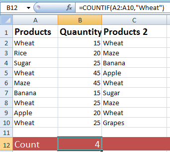
For getting the count for the duplicate values, you may use the Excel COUNTIF function. The COUNTIF function takes the range where you want to look up and the text that needs to be tested for duplication.

See the following example where I am using the same Excel sheet as in the above examples and getting the count of “Wheat” in the sheet. The COUNTIF formula is used as follows:

=COUNTIF(A2:A10,"Wheat")

The result:

A detailed tutorial is written about the COUNTIF in Excel.