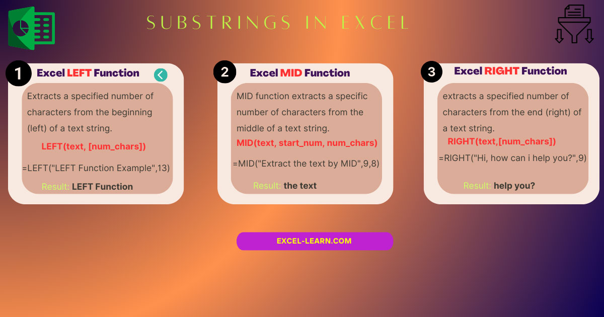
Functions to Get Substrings in Excel
The Excel has a few functions like LEFT, MID, and RIGHT that can be used for getting the substrings from the given text, specified cell etc.
In this tutorial, I will show you examples of using the functions to get substrings in Excel.
Excel has a few functions like LEFT, MID, and RIGHT that can be used for getting the substrings from the given text, specified cell, etc.
Excel LEFT function
For returning the first character or desired number of characters from the left of given text string, you may use the LEFT function.
The syntax of using the LEFT function is:
Where:
| Text | Text is the required argument. This is the text from where a substring will be returned. You may use cell reference or constant literal. |
| num_chars | The num_chars is an optional argument. This specifies the number of characters to return from the left of a given text string. |
| num_chars is omitted | If num_chars is omitted, the default 1 is used. That is, one character from the left is returned. |
- The num_chars must be greater than 1.
- If it exceeds the total length of the text, it returns the complete text string.
The example of getting substring by LEFT function
In the first example of the LEFT function, I am using a text string in the LEFT function and provide a number to get a substring. The LEFT formula:
The result:
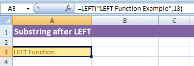
I applied this formula in the A3 cell and it returned “LEFT Function” substring.
What if num_char was omitted?
See the same example as above and this time I will not use the second argument i.e. num_chars. See the result and formula below:
The result:
The above formula only returned one character from the left i.e. “L”.
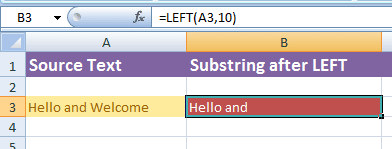
Using cell reference in the LEFT function
This time, I will use the cell reference (A3) in the LEFT function for the text argument. The returned substring will display in the B3 cell for num_char=10.
You may also use a cell reference for the num_char argument. For example:
In that case, enter the number in the A4 cell to get the substring from A3 cell.
Extract the substring by Excel MID function
The MID function can be used to extract the substring in Excel by providing the text string, starting number and number of characters to return.
The general syntax of the MID function is:
An example of MID function to extract the substring
I will use the text in MID function with start and number of characters arguments as follows:
The MID formula:
The result:
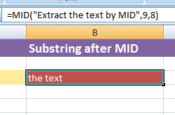
In the result, you can see the MID function started extracting the substring from the 9th character which is “t” and moved towards right till 8 characters.
Dynamically using MID function example
For this example, I will use cells for all the arguments in the MID function for extracting a substring.
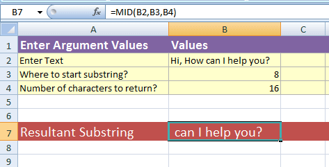
The Formula:
So, we are taking the source text from the B2 cell.
The start number is taken from the B3 cell while the B4 is used for the number of characters from the start number to return by MID function.
The RIGHT function in Excel to get substrings
The RIGHT function returns the substring from the right most of the text string. It also takes two arguments i.e.
If you omit the num_charc argument, the RIGHT returns one character from the right of the text.
An example of the RIGHT function
The following example gets the substring by using RIGHT function with both parameters.
The formula:
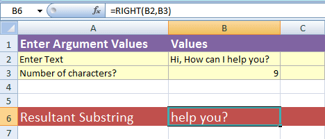
You can count and see it returned 9 characters that started from the right of the text (given in B2 cell).
If you do not provide num_chars argument then see the result by using this formula:
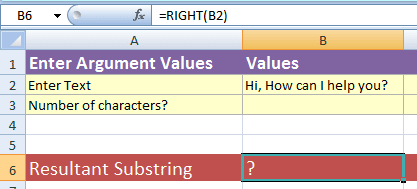
You see, it only returned the last character i.e. ‘?’.