TEXT Function in Excel
Explore eight practical examples of using the Excel TEXT function to convert numbers and dates to custom text formats.
Excel TEXT Function
- The Excel TEXT function can be used to convert numbers and dates into text.
- This is particularly useful for scenarios where you require displaying the numbers or dates with text strings.
- You may also use the TEXT function for formatting dates.
- Generally, the TEXT function is used with other functions. For example,
- 1. Syntax of using the TEXT function
- 2. A simple example of the TEXT function
- 3. Display the day name of today by TEXT function
- 4. Number with %, and two decimal points
- 5. Display leading zeros for a number example
- 6. Display a thousand separators in numbers
- 7. The example of date formatting codes in TEXT function
- 8. Format codes for time in TEXT function
- 9. An example of using TEXT function with CONCATENATE
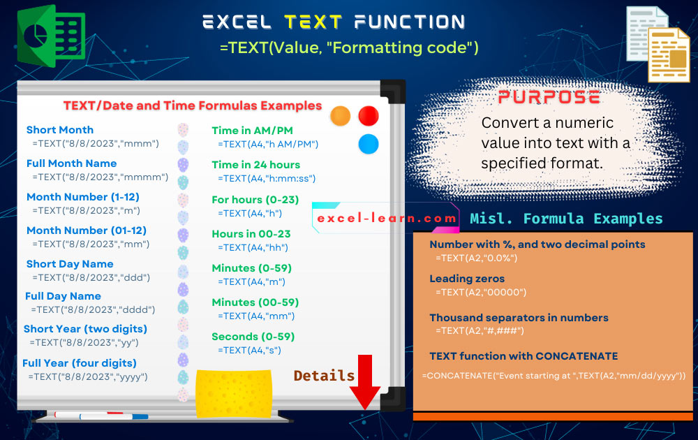
Syntax of using the TEXT function
The general syntax for using the TEXT function in Excel:
| Argument | Description |
| Value to convert into text | In the first argument, you may provide a number, date, etc. to be converted into the text. |
| Formatting code | The formatting code like decimal points in numbers, date format, etc. |
By using formatting codes, you may format dates and times as per the requirement and locale.
A simple example of the TEXT function
Let me start with a basic example of using TEXT function. In the A2 cell, a number is given while a date is given in the A3 cell. The TEXT function is used in B2 and B3 cells for converting the respective number and date into text:
The B2 formula:
The B3 formula:
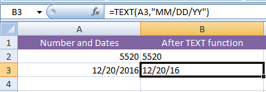
The evidence that both are converted to text is the display of number and date in B2 and B3 cells as left aligned. By default, the number and date are aligned right as in the case of A2 and A3 cells.
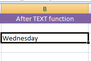
Display the day name of today by TEXT function
The following example used the TODAY() function to get the current date and displayed the day name e.g. Tuesday, Wednesday by using the TEXT function:
The TEXT formula:
The result:
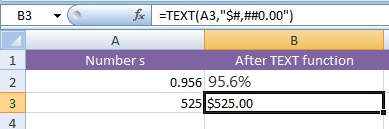
Number with %, and two decimal points
This example displays the specified A2 cell number with percentage and A3 cell with two decimal points with ‘$’ sign:
The formula for B2:
For B3:
The result:
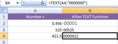
Display leading zeros for a number example
By default, Excel will not display leading zeros for the numbers. For example, if you try entering the number 00525, Excel displays it as 525.
The example below shows the leading zeros for numbers in different cells.
The TEXT formula:
You may use more or less number of zeros – depending on the requirement.
Display a thousand separators in numbers
This example displays the numbers with 1000 separators. You may use # or 0 in the formatting code as shown below:
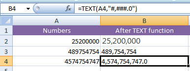
The formula used in B2 for A2 number:
The formula in B3:
In B4:
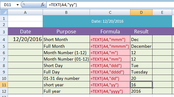
The example of date formatting codes in TEXT function
The following example shows using a few date formatting codes with the TEXT function.
For the example, I have used the “12/20/2016” date and by using the TEXT function formatting code argument, the month number, month name in three letters, full month name, the day with and without leading zero, day name in three letters and full day name are displayed as follows:
If you want to copy any of these formulas, these are listed below:
| Formula | Description |
|---|---|
=TEXT(A4,"mmm") |
Short Month (e.g., Jan, Feb) |
=TEXT(A4,"mmmm") |
Full Month Name (e.g., January) |
=TEXT(A4,"m") |
Month Number (1-12) |
=TEXT(A4,"mm") |
Month Number (01-12) |
=TEXT(A4,"ddd") |
Short Day Name (e.g., Mon, Tue) |
=TEXT(A4,"dddd") |
Full Day Name (e.g., Monday) |
=TEXT(A4,"dd") |
Day Number (01-31) |
=TEXT(A4,"yy") |
Short Year (two digits) |
=TEXT(A4,"yyyy") |
Full Year (four digits) |
Format codes for time in TEXT function
Similarly, you may use the format code argument in the TEXT function to display the time in your desired format. Like we used m, d, y variations for dates, the h, m, s, am/pm are used for time formatting.
The format code is case insensitive i.e. you may use h or H etc.
See the following example with various formulas used to display time:
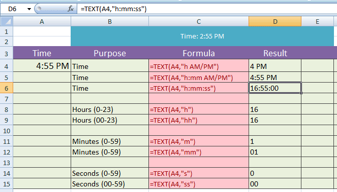
The following formulas are used for getting the time, hours, minutes, and seconds from the A4 cell (4:55 PM).
| Formula | Description |
|---|---|
=TEXT(A4,"h AM/PM") |
Time in AM/PM format (e.g., 3 PM) |
=TEXT(A4,"h:mm AM/PM") |
Time in AM/PM format with minutes (e.g., 3:15 PM) |
=TEXT(A4,"h:mm:ss") |
Time in 24-hour format with seconds (e.g., 15:30:45) |
=TEXT(A4,"h") |
Hours (0-23) |
=TEXT(A4,"hh") |
Hours in 00-23 format |
=TEXT(A4,"m") |
Minutes (0-59) |
=TEXT(A4,"mm") |
Minutes in 00-59 format |
=TEXT(A4,"s") |
Seconds (0-59) |
=TEXT(A4,"ss") |
Seconds in 00-59 format |
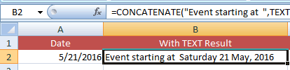
An example of using TEXT function with CONCATENATE
The example below shows using the TEXT function with the CONCATENATE function. For that, the date in A2 cell is converted to text and combined with a string by using the CONCATENATE function.
To show the difference, the B2 displays the result by simply joining the A2 date without the TEXT function:
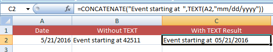
You see, the formatting of the date in A2 cell is removed in B2 as I simply used it in CONCATENATE function. The C2 displayed it correctly where this formula is used:
The formula in B2:
See another formula for displaying this date more elegantly:
The formula:
The result: