Doing Multiplication in Excel

There is no formal function like MULTIPLY in Excel for performing multiplications. You may use the ‘*’ operator for multiplying numbers, numeric cells in columns or rows, cell ranges etc.

You may simply use the ‘*’ operator e.g. 10*5, A2 * B2 or use the multiple operators in various functions. The PRODUCT function can also be used for multiplication of numbers and ranges. In the following section, I will show you examples of multiplying in Excel by different ways.

The example of multiplying two numbers

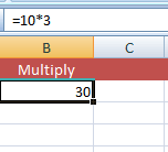
Starting with a basic example, let us display the result of two numbers after multiplication into the B2 cell. This is as simple as this:

=50 * 3

For that, type the ‘=’ followed by numbers e.g. 8 * 5 in the cell where you want to display multiplication result.

You may also select a cell and enter the formula in the formula bar e.g. =8*5.

Following mathematics rules as multiplying

See the following Excel sheet with results to understand the order of calculations as various operators like +, -, *, division etc. are used in different orders:

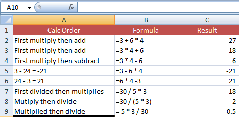
From the result, it can be concluded that Excel performs calculation in the following order:

• () Parenthesis
• % percentage
• * and / has the same precedence. Excel checks from the left and what comes first will be calculated.
• + and –

You may learn more about the order of calculation here.

The example of Excel multiplication in two cells

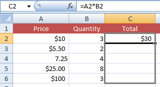
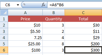
In the following example of how to multiply in Excel, column A is assigned the prices and column B contains quantity. Column C displays the total by multiplying A and B respective cells.

The formula applied to the C2 cell:

=A2*B2

Similarly, you may right =A3*B3 in the C3 cell and so on. In that case, you have to write the formula in C4, C5 etc. cells one by one with respective A and B cells.

The shortcut way of applying this multiply formula to all C cells can be as follows.

Write the =A2*B2 formula in the C2 cell and press Enter.

Now select the C2 cell and bring the mouse pointer to the right bottom of the C2 until + sign appears with the solid thin line.

Drag the fill handle to the desired cell and leave the mouse.

The formula should be copied in each C column cell while Excel will update the A and B column’s cells automatically.

How to multiply more than two cells?

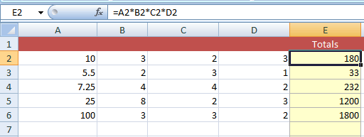
The following example shows multiplying four cells at a time. So, the formula for E2 that displays the calculated result is:

=A2*B2*C2*D2

The resultant sheet:

How to multiply rows?

If your data is arranged horizontally and you require multiplying rows data then following example demonstrates how you may do this:

Suppose, we have a number of products stored in row1 and Quantity in row 2. The row 4 should display the multiplied result:

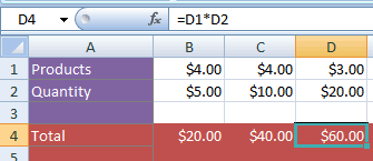
The following formula is applied to the B4 cell:

=B1*B2

Just like we multiplied columns data in above example and copied in other cells, you may select the B4 cell after writing this formula. Bring the mouse over the right bottom of the B4 cell until + sign appears with the solid line. Now drag the handle to the required row and leave it. The formula with respective row cells should be copied across (as in our example case; from B4 to D4 cell).

Using PRODUCT function for multiplication

You may also use the PRODUCT function for multiplication in Excel. The benefit of using PRODUCT function is it allows multiplying ranges apart from providing two or more cells independently.

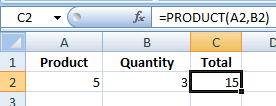
First, have a look at the formula for multiplying individual cells by using PRODUCT function:

=PRODUCT(A2,B2)

The result:

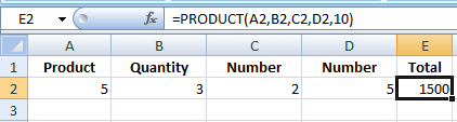
Similarly, you may provide more than two cells or numbers in the PRODUCT function for multiplication. For example:

=PRODUCT(A2,B2,C2,D2,10)

The result:

An example of using range in PRODUCT function

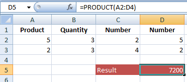
If you are tired of using individual cells for large data sets multiplication then you may use the range of cells in the PRODUCT function. See an example below:

The PRODUCT formula:

=PRODUCT(A2:D4)

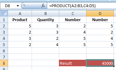
Of course, you may use multiple ranges in the PRODUCT function for multiplication. For example:

=PRODUCT(A2:B3,C4:D5)

The resultant sheet:

Using SUMPRODUCT function for multiplication and sum

As such, the PRODUCT function can be used for the multiplication of ranges. The SUMPRODUCT function can be used for getting the SUM of ranges after multiplication.

For understanding this function, consider this Excel sheet that we also used in above examples.

We used Price and Quantity columns and got its multiplied result. Now we also require the sum of all price/quantity cells after multiplication.

Just to remind, this is how we multiplied price and quantity in above example:

By using SUMPRODUCT function, see how it gets the sum after multiplication:

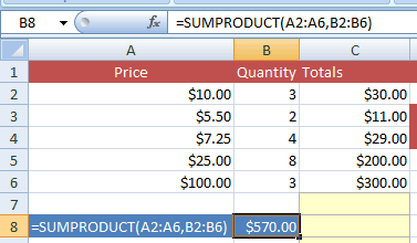
The SUMPRODUCT formula:

=SUMPRODUCT(A2:A6,B2:B6)

If you calculate the Totals in C column, it will produce the same result as returned by SUMPRODUCT function.