Excel INDIRECT Function
The INDIRECT function is used when you require changing the reference to a cell in a formula while you do not want to change the formula itself.

What is the INDIRECT function in Excel?
Generally, we write formulas in Excel with hard-coded cell references, range references, names, etc. For example:
- In the future, if you want to add more cells in the SUM function then you need to modify the formula.
- The INDIRECT function is used when you require changing the reference to a cell in a formula while you do not want to change the formula itself.
- Excel INDIRECT function allows to create dynamic references to cells, ranges, or named ranges.
- Sounds tough and boring? Hopefully, the examples coming up in the sections below will make it clearer and you will see its usefulness.
Syntax for using INDIRECT function
The general syntax of using the INDIRECT function:
Where:
| Argument | Description |
| ref_text | Ref_text is required. This is where you will specify the text string and the INDIRECT function returns the reference based on this.
The returned reference is immediately evaluated to display its content. |
| a1 | The a1 argument is optional. It has two possible values: TRUE/FALSE.
The default value is TRUE which means interpret ref_text as the A1-Style reference. The FALSE value means R1C1-style reference. |
A simple example to begin with INDIRECT function
The first example to understand how the INDIRECT function works is pretty simple.
In the Excel sheet, I assigned text to the A column cells, and in the B column, I used the INDIRECT function as follows.
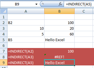
In the Excel sheet you can see these formulas with the results:
It displayed the value in the B2 cell because A2 cell contains the reference to B2.
Resulted in #REF! as A3 cell contains invalid cell reference.
Returned the B5 cell’s text.
Using the name reference
The following example shows using the name in the INDIRECT function. For that, I have given a name to the B5 cell and see the result.
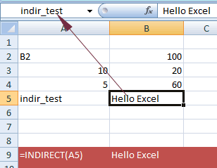
The formula:
As A5 contains “indir_test” that refers to the B5 cell, so it displayed the B5 value.
The example of using SUM and INDIRECT functions
In this example, we have two numeric columns. One contains the “Total Number of Sales” and the other contains the Amount. Both of these column’s cells are given names; Sales and Amount, respectively.
Next, I used the SUM and AVERAGE formulas to get the total of Sales and Amount range names. These are used in the INDIRECT functions as follows:
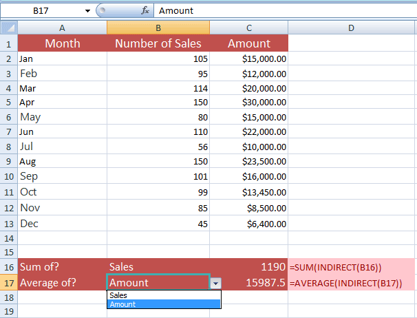
I have created two dropdowns that contain the names of ranges (Sales and Amount). The SUM/INDIRECT function refers to the B16 cell that contains the dropdown:
As you select Sale/Amount from the dropdown, its sum is displayed in the adjacent C16 cell.
Similarly, the AVERAGE/INDIRECT formula is used as follows:
Make sure that dropdown values contain the same name as the named ranges are, otherwise, #REF! error occurs.
Locking the cells example
One of the benefits of using the INDIRECT function is it can lock the cells. The advantage of this is in cases where you require inserting row(s) or columns after using the INDIRECT formula.
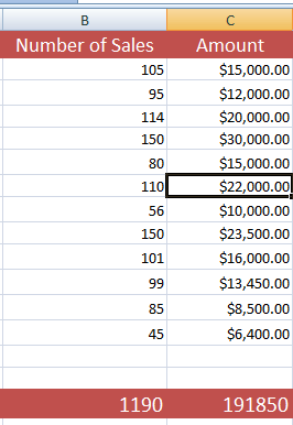
For example, in our Number of Sales and Amount columns, if we apply these formulas to get the sum:
To the Number of Sales and this is used to get the sum Amount:
The result is:
If we require inserting a row after the headers row on top with values then the SUM formula will adjust itself from:
To
Whereas, the formula with SUM/INDIRECT will be:
=SUM(INDIRECT("C2"):C14)
So, if you insert the values for Number of sales and Amount, the resultant sheet will be:
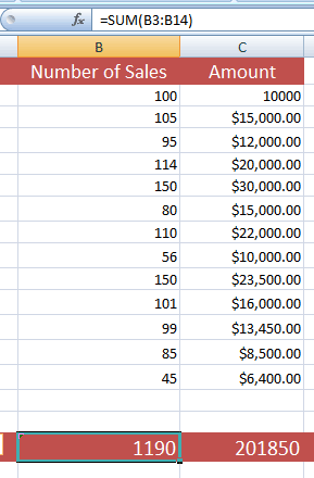
You can see that the Number of Sales new value (100) is not added to the total whereas the Amount is showing an addition of 10000.
Using INDIRECT function with different sheet example
You may also refer to some other sheet within the same workbook as using the INDIRECT function. See the simple formula where I used the sheet name in the INDIRECT function.
The INDIRECT formula for referring to another sheet:
In the formula, we referred INDIR sheet’s B2 cell.
You may also reference another sheet by referring a cell:
=INDIRECT(A2 & "!" & B2)
The result:
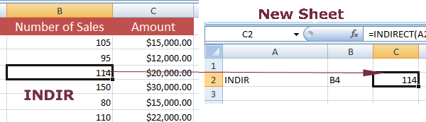
In the left sheet (INDIR), you can see B4 cell contains 114. In the INDIRECT formula, I referred A2 cell (in the new sheet) that contains INDIR value. This points to the other sheet we want to refer in the INDIRECT function.
The other part refers to the B2 cell in the new sheet that contains B4 value. Thus, the INDIRECT returned the B4 value in the “INDIR” sheet.
How to refer some other workbook sheet?
In the above example, we referred to another sheet in the same workbook. You may also refer to a sheet from some other workbook.
For that, you have to use the other workbook name, its sheet, and the cell reference that you want to get the value.
A sample formula is shown below:
=INDIRECT("'[" & A1 & "]" & B1 & "'!" & C1)
The sheet where this formula is used:
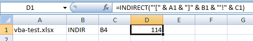
In this case, the A1 contains the workbook name, B1 refers to the “INDIR” sheet and C1 refers to the cell in the “INDIR” sheet.