How to use Count Function in Excel?
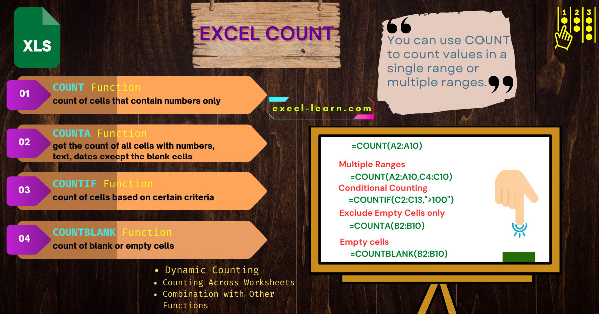
if you require the count of cells that contain numbers only, use the Excel COUNT function.
To get the count of all cells with numbers, text, dates etc except the blank cells, use the COUNTA function. Similarly, for returning the count of cells based on certain criteriause the COUNTIFS function. To get the count of blank or empty cells, use the COUNTBLANK function.
Count Functions in Excel
- To get the count of numbers, dates, text, and empty or non-blank cells, you may use various built-in functions in Excel.
- Depending on the requirement, you may choose which one to use;
- For example, if you require the count of cells that contain numbers only, you may use the Excel COUNT function.
- To get the count of all cells with numbers, text, dates, etc except the blank cells, use the COUNTA function.
- Similarly, returning the count of cells based on certain criteria e.g. count of cells that contain “A” can be done by the COUNTIF function.
- For multiple criteria use the COUNTIFS function. For example, return the count of cells that are between two dates.
- To get the count of blank or empty cells, use the COUNTBLANK function.
In the following section, I will show you Count Formulas in Excel with data in spreadsheets. You may copy any formula in your sheet to see how it works.
- 1. Get the count of numeric cells by the COUNT function
- 2. What if cells also contain dates?
- 3. Using multiple ranges in the COUNT function
- 4. Using Excel COUNTIF function for conditional counting
- 5. Getting the count of matched text
- 6. Using the '*' wildcard in the COUNTIF function
- 7. Using “>=” in COUNTIF for number count
- 8. Using “<” operator in the COUNTIF function
- 9. An example of Not equal to operator “<>”
- 10. Getting a count of multiple ranges by COUNTIF
- 11. The Example of using COUNTIF with dates
- 12. An example of COUNTA function
- 13. How to get the count of empty cells?
- 14. How to use COUNTIFS function
- 15. The example of using the Excel COUNTIFS function
- 16. Using three conditions in COUNTIFS
Get the count of numeric cells by the COUNT function
Let us start with a simple example of counting the number of cells that contain numbers only.
For that, I have filled cells from A2 to A10 with numbers, text, and blank cells. See what we get by the COUNT function:
The COUNT formula:
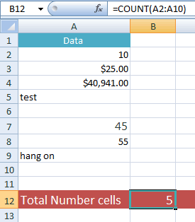
You can see that the COUNT function only returned the count for cells containing numbers. The blank and text cells are ignored while numbers with currency format are also included.
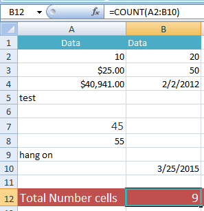
What if cells also contain dates?
The COUNT function also reruns the cells that contain dates. To demonstrate that, I extended the above range to the B10 cell and added two numbers and two dates in B cells.
So, the COUNT formula is:
See the figure with the formula and result:
Using multiple ranges in the COUNT function
Two things are further used in this formula.
- The first is using multiple ranges i.e. A2:A10 and C4:C8.
- The second thing tested whether the COUNT function returns the text with a number e.g. “6test”.
See the formula and output:
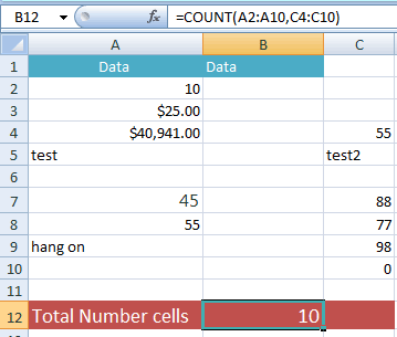
You saw the COUNT did not return “2test” occurrence.
You may provide up to 255 ranges, cell references, or items that you want to get the count.
Using Excel COUNTIF function for conditional counting
If you require getting the count of the number of cells based on a single criterion then use the COUNTIF function.
If you separate two words: “COUNT” “IF”, it makes the purpose clear.
For example, COUNT the cells from A2:D1000 IF that contains the word “Microsoft”. Similarly, return the number of cells whose date is less than or equal to 10/10/2010 and so on.
General Syntax of COUNTIF
You may provide a range of cells, array, names range, etc as the first argument.
In “What to search” argument, you will specify e.g.
- "London"
- A cell reference like A10
- “>1” count the cells whose value is greater than 1
- “<=10” less than or equal to 10
The next section shows a few examples of using the Excel COUNTIF function.
Getting the count of matched text
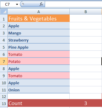
In this example, we will get the count of “Apple” in our example sheet. The column A cells contain the Fruits and Vegetable names. In the COUNTIF function, I specified the Apple as follows:
=COUNTIF(A2:A11,"Apple")
The result:
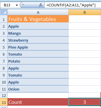
You can see the text Apple occurred three times in the given range.
Using the '*' wildcard in the COUNTIF function
You may also use the wildcards (* and ?) in the COUNTIF function. The '*' is used for any sequence of characters while the '?' mark is for a single character.
In the following example, I used the “to*” in the COUNTIF for the same sheet as used in the above example and see the formula and result:
The COUNTIF formula:
The result:
You saw the occurrences of Tomato (twice) and Potato (once) is returned as 3.
Using “>=” in COUNTIF for number count
For this example, I will use the single criteria for counting the cells containing the number of sales greater than or equal to 100 in the COUNTIF function.
For this example, the Excel sheet contains month names in B cells and a number of sales in C cells. The following COUNTIF formula is used:
The resultant sheet:
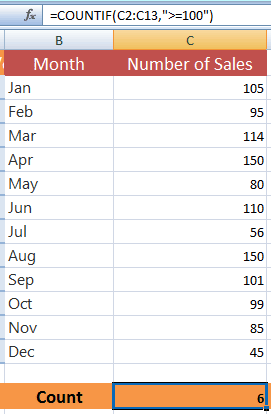
If you count the number of sales greater than or equal to 100, it is 6 that COUNTIF returned.
Using “<” operator in the COUNTIF function
Now, we will get the count of the Number of Sales less than 100 by using the COUNTIF function. The following formula is used:
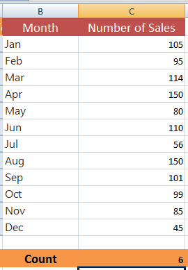
The count is again 6.
An example of Not equal to operator “<>”
For this example, I used the Not Equal to operator which is “<>”. The criterion set in the COUNTIF is to return the number of sales not equal to 150 i.e.
Result:
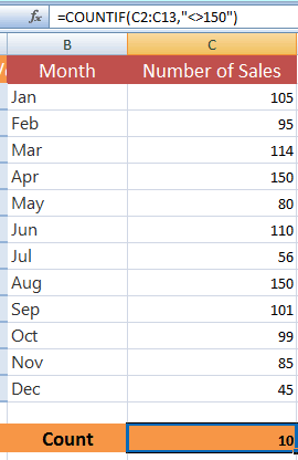
If you look at the data in the Excel sheet, it contains 150 twice. So, the COUNTIF omitted these and returned 10 counts.
Getting a count of multiple ranges by COUNTIF
In this example, we will get the count of two different ranges by using the COUNTIF function twice and adding the returned result.
For that, I have added another column in the above sheet i.e. Amount.
By using the COUNTIF function, we will get the count of (number of sales more than 100) + (Sale amount greater than or equal to $15000). See how this is translated into COUNTIF:
The returned result:
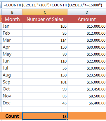
If you count the C cells (C2:C13) then the count of cells with more than 100 sales is 6.
Add this to the count of D2:D15 cells with the amount greater or equal to 15000 then it is 7. The sum of both returned values is 13.
You may use more than two COUNTIF formulas as well. The function of using multiple conditions/criteria is COUNTIFS which is coming up in next sections.
The Example of using COUNTIF with dates
Just like the numbers, you may also write a criterion for date columns to get the count. For example, get the count of employees who joined after 3rd Jan 2012.
To demonstrate the usage of dates in the COUNTIF function, I am using an Excel sheet containing fictitious records of employee names and their joining date.
A named range is created which is referred in the COUNTIF function.
By using COUNTIF function, we will get the:
- Total count of employees
- Number of employees who joined after 2010
- Number of employees who joined before 2007
- and the employees who joined between 2008 to 2012.
First, have a look at the resultant sheet which is followed by COUNTIF formulas:
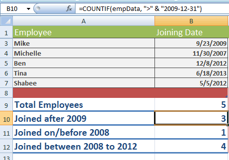
The formula to get the total number of employees:
Where empData is the range name containing cells A3 to B7.
The COUNTIF formula for getting the number of employees joined after 2009:
Joined on or before 2007:
Joined between 2008 to 2012 formula:
The last formula used COUNTIFS as we have two conditions to check. I will explain this in the COUNTIFS section.
You may learn more about the COUNTIF function in its tutorial: Using COUNTIF function.
An example of COUNTA function
The COUNTA function will only omit the empty cells. See the following example, where I have used different types of values in an Excel sheet and used the COUNTA function to get the count:
The COUNTA formula:
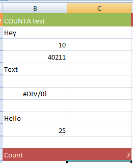
You can see that the resultant sheet displayed count equal to 7 as two cells in the given range are empty.
How to get the count of empty cells?
Have a look at the same Excel sheet and data as used for COUNTA function for demonstrating the COUNTBLANK function.
The Excel COUNTBLANK formula:
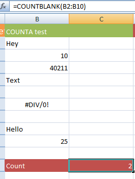
The returned count is 2 as you can see the given range contains two blank cells.
How to use COUNTIFS function
As mentioned earlier, if you have multiple criteria to check for getting the count in a range, array, etc. you may use the COUNTIFS function.
For example, return the count of those employees who joined after 10/20/2012 and their salary is $5000 or above.
We have seen that COUNTIF enables using a single criterion only whereas COUNTIFS allows us to get the count based on multiple criteria.
The example of using the Excel COUNTIFS function
For the example of the COUNTIFS function, I am using the same Excel sheet as used in an above example that contains Months, Number of Sales, and Amount columns.
The requirement is to count those rows in which Number of Sales is greater than or equal to 110 and amount >= $15000.
The COUNTIFS formula is:
The result:
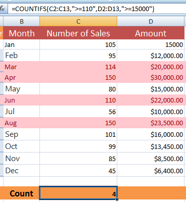
You can see, the highlighted rows met both criteria. If you look at the first row, the amount is $15000 which is true, however, the number of sales is 105 which is False; so COUNTIFS did not include this row.
Using three conditions in COUNTIFS
In this example, I am using three conditions in the COUNTIFS. For that, extending the above formula and another criterion is added to return the count of those rows that start with the month “J”. While the number of sales is set as greater than 100.
The COUNTIFS formula:
The result:
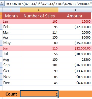
You see, I used ‘*’ wildcard as the first criteria i.e. B2:B13,"J*". If you go through the table, only two highlighted rows met all the criteria given in the COUNTIFS function.