What is a Pivot table?

For understanding the concept of Pivot tables, suppose we have a large Excel table containing hundreds of records for sales made by salespersons on monthly basis.

The spreadsheet or Excel table contains Salesman ID, Name, Month, Product and number of sales made in that month. Now, going through hundreds of records for making important business decisions like the performance of salesman, getting average monthly sales for a specific product etc. can be a tedious task.

The Pivot table enables creating another table based on above table data and can summarize data for analysis like averages, sum, or other useful reports. With the Microsoft Excel pivot table feature, this is the matter of few clicks for creating a pivot table based on an Excel sheet or table and even you may create Pivot charts for further visualizing the data that updates as the main table is modified.

How to create Pivot table in Excel?

For demonstrating how to create Pivot tables in Excel, I am using the above mentioned table that contains fictitious records of salespersons as shown below.

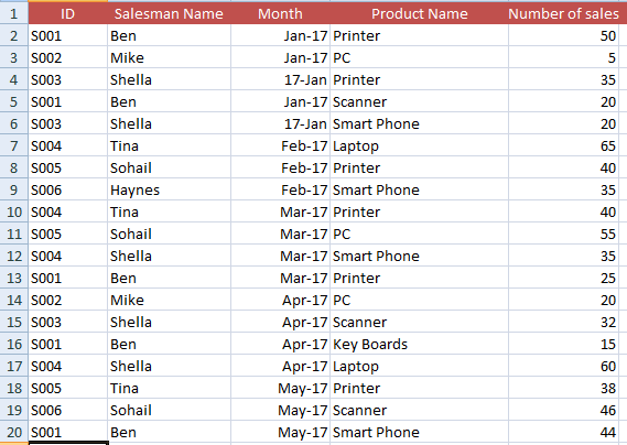
You can see, the table contains ID, Name, Month, Product Name and Number of Sales. On the basis of this table, we will create Pivot table by following these steps:

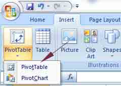
Step 1:

Select any cell in the table and go to the “Insert” in the Ribbon. Find and press the “Pivot Table” in the Table group. Depending on the Excel version (2007, 2013, 2016), it may vary a bit but functionality remains the same.

Step 2:

The “Create Pivot Table” dialog should appear that automatically selects the current table’s range that will be used for the Pivot table:

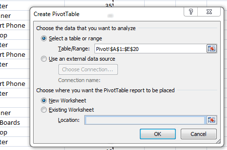
You can see the dialog box is already populated by cells range:

Pivot!$A$1:$E$20

You may change this if you require using the subset of data from the main Excel sheet/table. I will use the complete data set for the demo.

The next option is “Choose where you want the Pivot Table report to be placed”. As I selected a cell inside the main table, the “New Worksheet” option is pre-selected.

If you select an empty cell before opening the “Create Pivot Table” dialog, the “Existing Worksheet” will be selected by default. Anyways, you may specify the target location there. I am using “New Worksheet” for the demo and press OK.

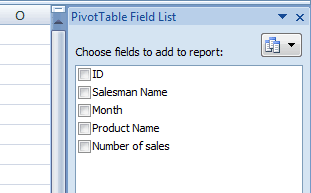
The Pivot table should be created in new Excel sheet with certain options as shown below:

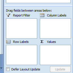
[stextbox id='info' bwidth='2' color='f7f5f5' bcolor='c4bb8b' bgcolor='171f07' bgcolorto='2c6134']By default, Excel adds the non-numeric fields in the Row area. The numeric fields are added in the Values area whereas the date & time fields are added to the Columns area.[/stextbox]

Creating First Report: Total Sales by salesman

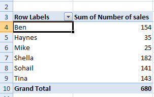
Now, let us see the magic; how helpful Excel Pivot table is. The first report that we want to look at; how many sales are made by each salesman for all time.

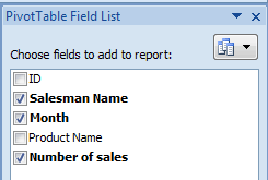
For that, go to “Choose fields to add to report” window (should be located towards the right side, as shown in above graphic). These windows give different views of the underlying table by a few clicks.

As you select “Salesman Name” and “Number of Sales”, the Pivot Table should display the following report:

The monthly sales report by salesman name

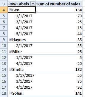
The above report displayed the accumulative sales reports for each salesman for all time. Now, we require monthly sales report for each salesman grouped. For that, simply add the “Month” field:

And there we go, the report is ready as shown below:

A report by Product Names for each Salesman

Similarly, you may generate a report based on Product Names for each salesman by selecting the Salesman Name, Product Name, and Number of sales fields as follows:

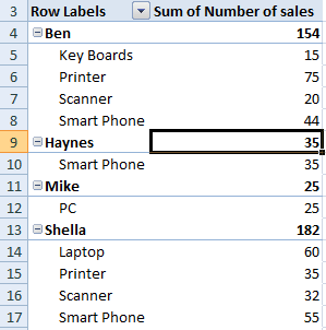
You can see how clear the report is for each salesman’s sales for product names.

Sorting the Pivot table example

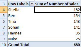
After creating a report, you may sort the results easily. For example, we created a report for the total number of sales by each salesman as shown below:

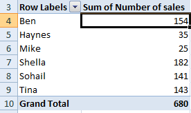
Now, we want to sort this report by the highest number of sales to lowest. For that, right-click on any “Sum of Number of sales” cell and locate the sort option.

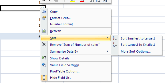
Press the “Sort Largest to Smallest” option and you will get the report sorted as shown below:

Similarly, if you select a salesman cell and right click --> sort, you may see “Sort A to Z” and “Sort Z to A” options for sorting the report in ascending or descending order.

Using the filter option example

You may require viewing the report of a specific salesperson only. For that, you may use the Filter option. Just drag a field that you want to enable filtering in "Report Filter" area:

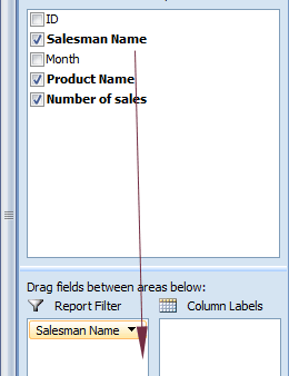
If your source data is an Excel table (which is recommended for creating Pivot tables) then the filter option should be available as the list shown below.

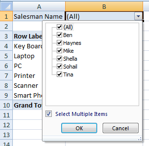
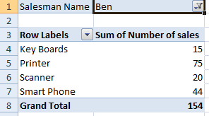
Let us say, we require the total sales made by Ben categorized by product names. For that, select the Ben in the list and see how Excel displays the report in Pivot table:

How to change the Summary calculation

We have seen the default summary for calculation is the sum of number of sales. In certain scenarios, you may require the count, average or some other calculation summary in the reports of Pivot table.

For example, in our example table let us get the count of the number of times a product name occurs for each salesperson.

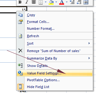
To change the calculation from the sum to count, right click on any cell that displays the “Sum of number of sales”.

On the context menu, click the “Value Field Settings”:

In the Value Field Settings dialog, select the Count option under the “Summarize value field by”. Press OK and see how the report is displayed now:

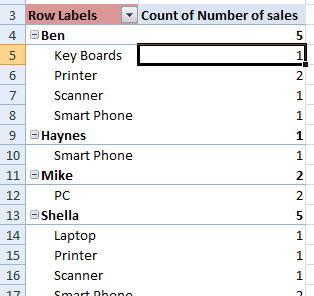
You can see, the count of product names is displayed for each salesperson.