Protecting Cells in MS Excel
In this tutorial, you will learn how to password protect a cell, multiple cells, a row and multiple rows in MS Excel.
In this tutorial, you will learn how to password-protect a cell, multiple cells, a row, and multiple rows in MS Excel.
So that the worksheet that you share can be edited for certain parts while others are protected.
How does cell protection work in Excel?
By default, all cells are “Locked” by Excel in a worksheet. You can see that as follows.
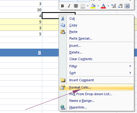
Right-click on any cell in the worksheet and click on the “Format Cells” item.
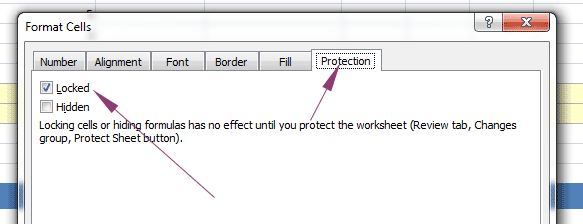
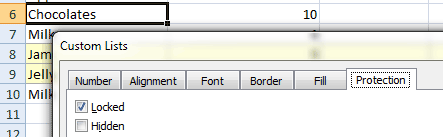
In the Format Cells pop up window, press the “Protection” tab as shown below:
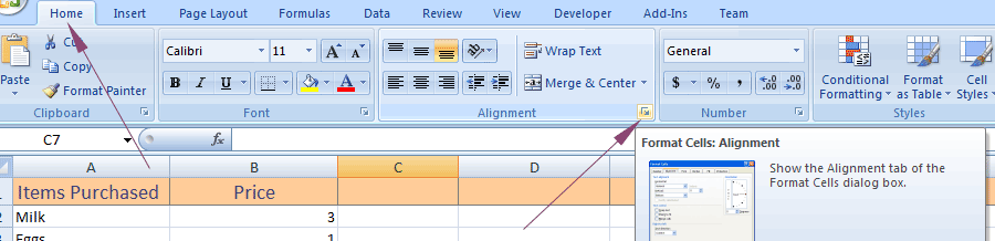
You may also access the “Format Cells” pop up window by doing the following:
Go to the “Home” in the ribbon and find the “Alignment” group. Click on the small icon for opening the “Format Cell” dialog box.
In the Protection tab, you can see the “Locked” option is already checked.
However, the data in the cells is still editable unless you do the further steps mentioned in the examples below.
Pro tip: The shortcut key for protecting/unprotecting the cells:
If cells/sheet is unprotected then it will ask to enter the password for protecting the worksheet.
If it is protected then the shortcut will open the popup for entering the password for removing protection.
Protecting the whole worksheet example
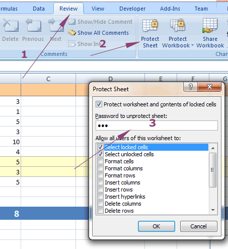
For protecting the whole sheet:
Go to the Review tab in the ribbon and click on the “Protect Sheet” under the “Changes” group.
Unprotect the sheet
After you lock/protect a sheet by entering a password, to make it editable for yourself and others, you need to unprotect it.
For that, go to the:
- Review Tab in the ribbon
- Click the “Unprotect Sheet”
- Enter the password that you set to protect the sheet
Protecting a single-cell example
For protecting a single cell, follow these steps (mentioned above as well with screenshots).
Select all cells.
Open the “Format Cell” pop-up by right-clicking on any cell and clicking the “Format Cells” option.
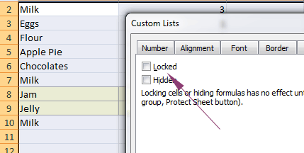
Under the “Protection” tab, uncheck the “Locked” checkbox. It makes all cells unlocked.
Suppose, we want to protect A6 cell only. Right-click on it and again open the “Format Cells” pop-up window.
Tick the “Locked” checkbox and press OK.
Now, go to the “Review” tab in the ribbon, and in the “Change” group, click “Protect Sheet”.
Enter the password as shown in the above section.
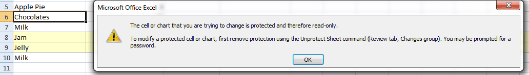
The A6 cell should be password-protected now while all other cells should be editable. If you try editing the A6 cell, this dialog should appear:
Making the heading row password-protected
It’s generally the header or specific cells with certain headings that you want to protect and do not want other users changing their content.
In order to make the top row that contains headings or titles of the columns protected follow the above step of unlocking all cells.
Then select the first row and go to “Format Cells” and tick the Locked checkbox.
Finally, go to the Review --> Protect Sheet and set the password there.
Locking and protecting multiple rows and cells
Similarly, if you want to lock and password-protect multiple rows or two or more cells, select those rows and cells (after unlocking all cells/rows).
Only lock the desired rows/cells.
Go to the “Review” tab and click on the “Protect Sheet” and set a password there.