How to subtract in Excel?
There is no Excel SUBTRACTION function. Instead, you may accomplish the task of subtracting numbers or a cell’s value from the other by using the minus arithmetic operator (-).
There is no Excel SUBTRACTION function. Instead, you may accomplish the task of subtracting numbers or a cell’s value from the other by using the minus arithmetic operator (-). For example:
=100-50
= B5 - A5
For subtracting numbers in cell ranges, you may use the SUM function. In that case, the cells containing negative values will be subtracted. See the following section for using the minus operator in different examples.
The example of subtracting numbers
For subtracting numbers, you may directly write the numbers with minus sign in the desired cell. Alternatively, go to the formula bar and right the numbers for subtraction as shown below:
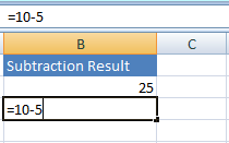
You can see, the numbers are typed directly in the cell preceded by the ‘=’. The Excel will subtract the numbers and display the result in that cell.
=10-5
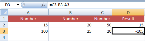
An example of subtracting cells numbers
The following example displays the subtracted result of three cells (A, B, C) in the respective D cells.
The subtraction formula in the D3 cell:
=C3-B3-A3
The resultant sheet:
The order of calculation
The Excel follows the calculation order if you are using multiple operators in the formula. The following order is used for calculation:
- Parenthesis
- Exponents
- / and * (which comes first from the left)
- + and – (that comes first from the left)
For learning more about Excel’s order of calculation, you may read the details here.
See an example below where I used multiple operators for calculation.
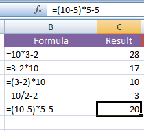
In formulas where parenthesis is used, Excel first subtracted and then multiplied.
=(3-2)*10 = 10
Without parenthesis, through subtraction came first from the left, it was first multiplied and then subtracted.
=3-2*10 = 17
The example of subtracting a range of cells
If you simply require viewing the calculation of multiple cells that contain negative and positive numbers then select the range of cells and look at the Status bar in Excel. The Excel automatically displays the sum, count, and average of selected cells as shown in the graphic below:
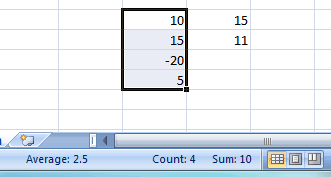
You can see, the cell contains negative and positive numbers. The sum is returned by subtracting the negative number.
Using the SUM function
For displaying the result in the specified cell, you may also use the SUM function of Excel. In that case, the cells containing minus numbers will be subtracted. See the example below:
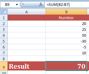
The sum formula for subtraction of numbers:
=SUM(B2:B7)
You can see, theExcel SUM function returned the result after subtracting the negative numbers.
The example of subtracting percentage
The following example shows the subtraction formula for subtracting the given percentage from a number. For that, the numbers are given from B2 to B6 cells. A percentage to subtract is given in C2 to C6 cell. The D2 to D6 display the result after subtracting the percentage:
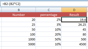
The formula for the D2 cell:
=B2-(B2*C2)
The formula is copied from D2 to D6 cells while Excel replaced the B2 and C3 respective cells automatically. For copying the formula, write the complete formula in D2 cell. Now bring the mouse pointer to the right bottom of D2 cell until + sign appears with solid line. Drag the handle down to D6 cell and you will see the results corresponding to B and C values.
Subtracting two dates example
The following example shows subtracting two dates by using the minus arithmetic operator. The Start and End dates are given in A2 and B2 cells. The C3 displays the difference as the number of days by simply subtracting two dates:
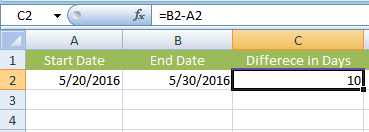
The formula is as simple as we used for subtracting two numbers:
=B2-A2
Subtracting given number of days/months and years from a date
The example below uses the DATE function for subtracting five years, five days and five months from the given date.
The date subtraction formula:
=DATE(YEAR(B2) - 5, MONTH(B2)- 5, DAY(B2) - 5)
The result:
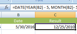
You can see, the given date 5/30/2016 is subtracted and the result is 12/25/2010.
You may learn more about date subtraction in its detailed tutorial: Subtracting dates in Excel.
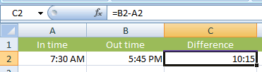
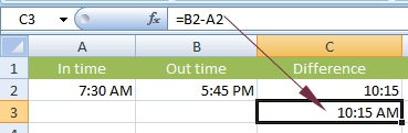
The example of subtracting time
You may also use the minus operator for subtracting time and get the difference in hours, minutes and seconds between two given times.
In this example, the cell A2 is given 7:30 AM and cell B2 5:45 PM. The C2 displays the difference in hours and minutes by using this simple formula:
=B2-A2
The result:
By default, the Excel displays time like this:
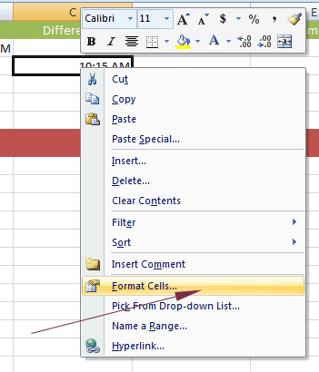
For displaying the result as hh:mm only, you need to format the cell. For that, right-click on the cell where you are displaying the result and click ‘Format Cells’:
In the “Format Cells” dialog, under the “Number” tab, select “Custom” and towards the right pane, select h:mm:
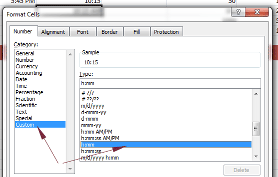
This should display the difference in time with hours and minutes without AM/PM.