How to use Excel SUMIFS for multiple criteria

In the SUMIF function tutorial, we learned how to SUM a range or cells by single criteria. The Excel SUMIFS function is used if you need to apply multiple criteria to get the sum of range.

An example of SUMIFS function

To explain the SUMIFS function, consider we have a table storing Items Purchased, Quantity and their Prices. (See the graphic with example data and formula below)

Now we want to calculate the sum of cells that contain Product Name “Milk” and which Total Price is greater than 4. So, we have two conditions to apply and this can be done by using SUMIFS as follows.

The SUMIFS formula:

=SUMIFS(C2:C10, A2:A10, "=Milk", C2:C10, ">3")

The excel sheet with data and result:

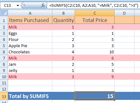
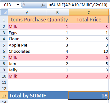
You can see, the highlighted rows show the occurrences of Milk three times. However, the SUMIFS returned the sum of only two cells i.e. 15. The cell with value 3 is omitted as it failed for one criterion.

Syntax of SUMIFS Excel function

On the basis of above example, let me explain the syntax/arguments of the SUMIFS function:

SUMIFS(sum_range, criteria_range1, criteria1, [criteria_range2, criteria2], ...)

Where:

The sum_range specifies the range where sum will be calculated. In our example case, the C2:C10 (Product Price) column was used because we needed the sum of price. This is required argument in SUMIFS.
criteria_range1 is the range where first criteria or condition will be checked. In the example, we specified the Item Purchased column from A2:A10. This is also required argument.
The third argument, criteria1 relates to the criteria_range1. This criterion will be checked for the criteria_range1. In the example, we checked “=Milk” for A2:A10 range. This is the required argument as well.
[criteria_range2, criteria2], ... This is optional and defines the second, third, and so on ranges and respective criteria in SUMIFS function. The allowed number of range/criteria is 127. In the example, I used second range and criteria as well. The second criterion was to check the Product Price > 3 i.e. C2:C10, ">3".

Be careful, as you are comparing SUMIF and SUMIFS function. In SUMIF function, the sum_range is given as the third optional argument while the single criterion is given as the second argument. See an example below.

The SUMIF function for a quick reminder

The following example shows using the SUMIF function so you have quick idea how different is the syntax or order of arguments in both function; to avoid mixing up both.

The SUMIF allows getting the sum based on single criteria as shown in the same excel table that I used in above example:

The formula:

=SUMIF(A2:A10,"Milk",C2:C10)

The resultant sheet:

Using a wildcard in SUMIFS with three criteria example

For this example, I will use the ‘*’ wildcard to find the sum of quality for the products which names starts with ‘A’. In the SUMIFS formula, I used three criteria to find the sum of quantity as follows:

The SUMIFS formula:

=SUMIFS(B2:B12, A2:A12, "=A*", B2:B12, ">1", C2:C12,">=4")

The resultant sheet:

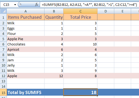
The sum to be calculated from the Quantity column, so B2:B12 range is given.
The first condition checked the Product Names that start with letter ‘A’ (A2:B12).
The second criterion is to check if Quantity is greater than 1, include this in the sum (B2:B12).
While the third condition checked the Product Price must be greater or equal to 4.
Only two cells fulfilled those criteria (B6 and B12) so returned sum is 18.