Excel SUBTOTAL Function
The SUBTOTAL function in Excel is used to return the subtotal in terms of sum, average, count, max, min etc. for the specified list, named range or database.
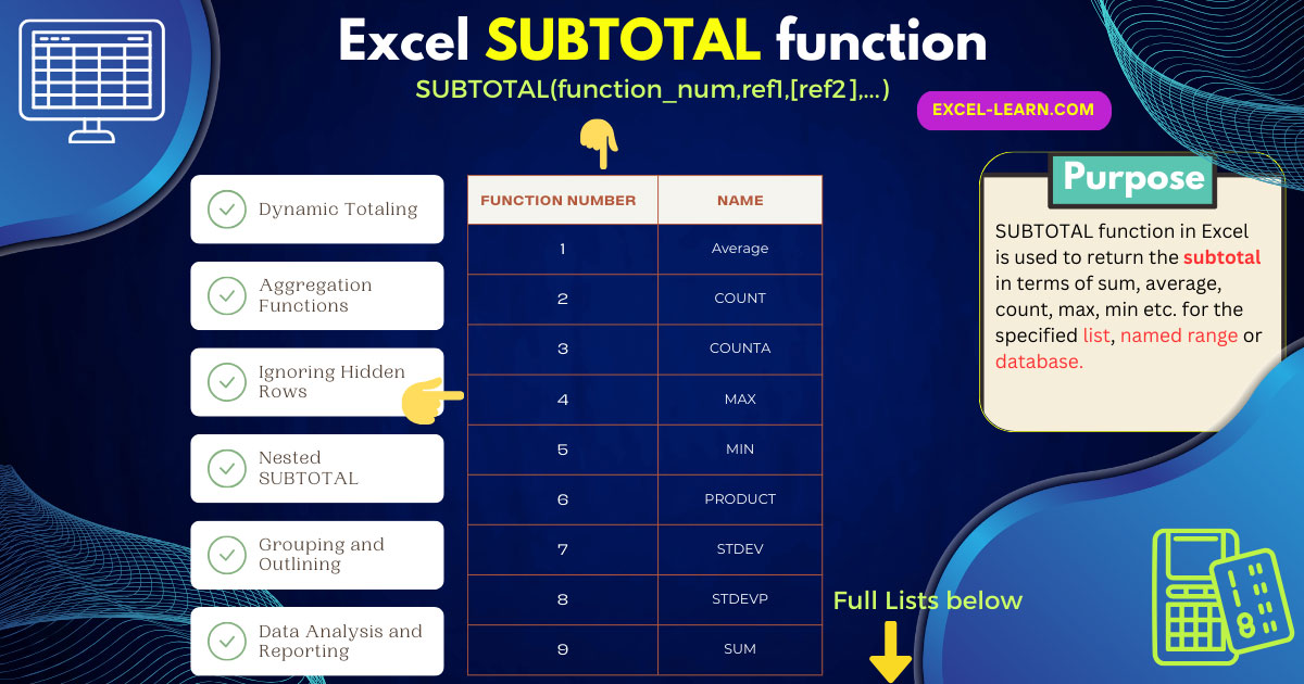
Purpose of Excel SUBTOTAL function
- The SUBTOTAL function in Excel is used to return the subtotal in terms of sum, average, count, max, min, etc. for the specified list, named range, or database.
- In the SUBTOTAL function, you have to enter the value of the function that specifies what is required as the subtotal.
- For example, the value 1 is for returning the average for the specified list or database and the value 9 means returning the SUM.
- See the full lists in the section below.
An example of SUBTOTAL to get the sum
Before explaining the syntax of SUBTOTAL, let us have a look at a simple example of using the SUBTOTAL function to get the sum.
For that, we have an Excel sheet with three columns that contain the Month, Number of Sales, and Amount. We will get the sum of B2:B5 range by using the SUBTOTAL function.
The SUBTOTAL formula:
The resultant sheet:
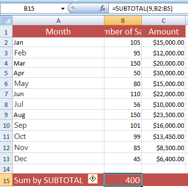
The value 9 means to return the sum of the given range. On the basis of this example, let us have a look at the general syntax of the SUBTOTAL function.
Syntax of SUBTOTAL function
SUBTOTAL(function_num,ref1,[ref2],...)
Where:
| Argument | Description |
| Function_num | Function_num specifies the function to use for the given range in the SUBTOTAL function. You may use 1-11 or 101-111 values in this argument.
The value 1 is for the AVERAGE function, 2 for COUNT, and 9 for SUM function.
See the list below to learn which function each of these numbers represents. This is the required argument in the SUBTOTAL function. |
| ref1 | The ref1 argument represents the reference, range, or named range, etc. I used B2:B5 in the above example, so SUBTOTAL returned the sum of that range only.
This is also a required argument. |
| ref2 | Optionally, you may also provide ref2 for the second reference or range.
The SUBTOTAL allows up to 254 references that you want to get SUBTOTAL. |
List of Function_num argument values with functions
Following are the numbers and respective functions that you may specify in the SUBTOTAL function:
Include hidden cell values
| Function Number | Function Name |
|---|---|
| 1 | Average |
| 2 | COUNT |
| 3 | COUNTA |
| 4 | MAX |
| 5 | MIN |
| 6 | PRODUCT |
| 7 | STDEV |
| 8 | STDEVP |
| 9 | SUM |
| 10 | VAR |
| 11 | VARP |
List of values that do not include hidden cells in SUBTOTAL function:
| Function Number | Function Name |
|---|---|
| 101 | Average |
| 102 | COUNT |
| 103 | COUNTA |
| 104 | MAX |
| 105 | MIN |
| 106 | PRODUCT |
| 107 | STDEV |
| 108 | STDEVP |
| 109 | SUM |
| 110 | VAR |
| 111 | VARP |
The example of getting average, max, and min values
The following example uses the Amount column in our example sheet to get the average, count, max, and min values for a given range. Have a look at the results and formulas:
The Excel sheet:
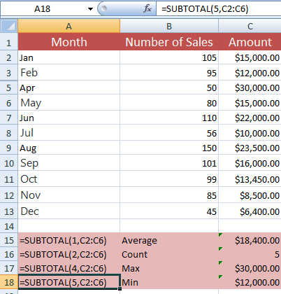
You can see that the month of March record is kept hidden (compare it with the above graphic). It contains the amount $20000.
The formula for getting the average:
For Count:
For maximum value in the given range:
For getting the minimum value:
Play with various function values in an interactive Excel sheet online
Below, you can see an interactive Excel sheet that contains the same data as used in the above examples.
You may interact with it right here or download it on your system. I have used the following generic formula in B16 cell:
As you enter a value in the B15 cell from 1-11 or 101 to 111, the respective formula will be applied to the B2:B7 range that contains the number of sales.
To see the difference between hidden and unhidden row values, I have hidden the third row that contains 150 values i.e. March record.
Enter various values within the limit in the B15 cell and see how it is updated in the B16 cell.
Using multiple ranges example
In the following example, I have used two different ranges in the SUBTOTAL function. The first range is B2:B4 and the second range is B11:B13. The SUBTOTAL formulas are used to get the sum, average, count, min, and max values as follows:
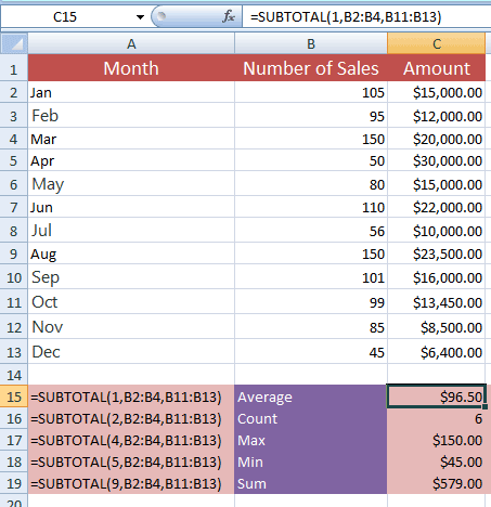
The following formulas are used:
Average:
Count:
Max:
Min:
Sum:
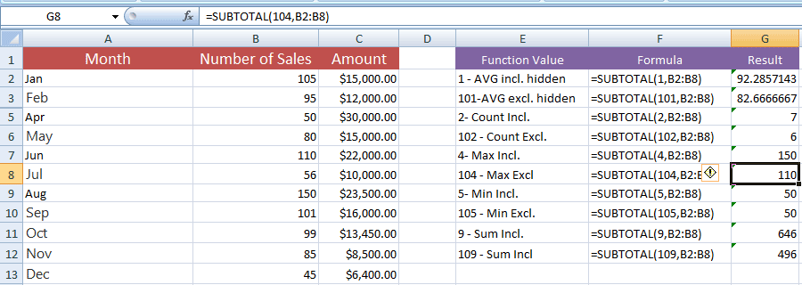
The following example shows the difference between different values for hidden and unhidden states of the rows.
For that, I have hidden the March row again that contains 150 values. In the E column cells, I displayed the formulas used for hidden and unhidden e.g. 1 for getting an average including hidden cells and 101 for excluding hidden cells.
The results are displayed in the G column for the same range i.e. B2:B8 so you can see the difference.