A brief about show/hide formulas in Excel
In this tutorial, you will learn how to show or hide the formula in the cells and formula bar in Excel.
You may require show or hide the formula for different situations. For example, by default Excel does not show the formula in the cell where you applied it. You may want to show it in the formula bar as well as in the cell.
Similarly, the formula is visible in the formula bar and if your Excel sheet is to be shared with teammates or publicly, you may want to hide the hard-written formula in the formula bar as well.
In this tutorial, you will learn how to show or hide the formula in the cells and formula bar in Excel.
Show the formula in a cell example
You may display the formulas in cells instead of their calculated values by using this shortcut:
Press CTRL + ` (grave accent)
Basically, this short key switches between displaying the formula and its result in the cell.
By the main menu
The same result can be achieved by using the main menu as follows:
Step 1:
Go to the Formula tab on the ribbon.
Step 2:
Locate the “Show Formulas” toggle button towards the right side.
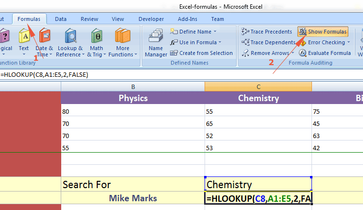
If you press it, it will display the formula in the cell. Upon pressing it again displays the formula result.
How to hide formula in the formula bar?
By default, Excel shows formulas in the formula bar. As mentioned earlier, if you share the spreadsheet with other users, they may view the formula written by you.
In order to hide it, follow these steps.
Step 1:
Select a cell or range of cells (adjacent or non-adjacent) for which you want to hide the formula.
Step 2:
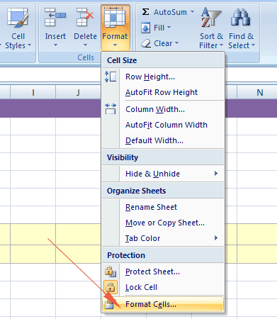
Go to the “Home” menu in the ribbon. Then locate the “Format” --> “Format Cells” as shown below:
A pop window should appear with a number of tabs. Go to the “Protection” tab and check the “Hidden” option.
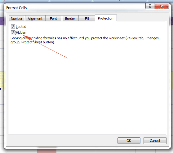
Click the Ok button.
No, the formula should still appear in the formula bar; you are not done yet!
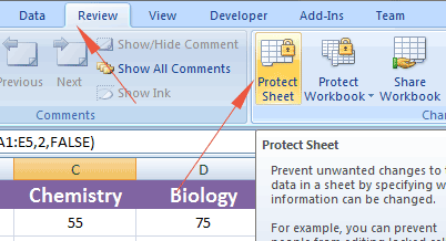
Step 3:
Now go to the “Review” in the ribbon and there locate the the “Protect Sheet”:
Another pop-up window should appear i.e. “Protect Sheet” as shown below.
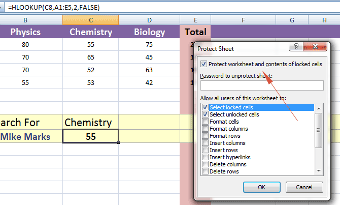
The “Protect worksheet and contents of locked cells” option should already be checked. If not make sure you check this and press the Ok button.
Now you should not see the formulas in the formula bar for the selected cell(s).
The “Protect Sheet” button under the “Review” tab should have become the “Unprotect Sheet” after executing the above steps.
In order to display the formulas again, just click the “Unprotect Sheet”.
Show/Hide formulas for various worksheets
If your workbook contains two or more worksheets and you want to display formulas instead of values in two or more worksheets then you may also set this option by following the steps below.
Step 1:
Click on the “Office” button towards the top-left or click the “File” (depending on your Excel version). Under this menu, click on the “Options” or “Excel Options”.
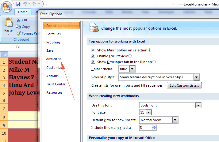
Step 2:
The “Excel Options” pop up window should open. There, click on the “Advanced” as shown below:
Step 3:
The “Advanced” window is long. Scroll down and locate the “Display options for this worksheet:”.
The dropdown next to this option should display the current worksheet. Select the worksheet that you want to display the formulas and check this option below:
“Show formulas in cells instead of their calculated results”
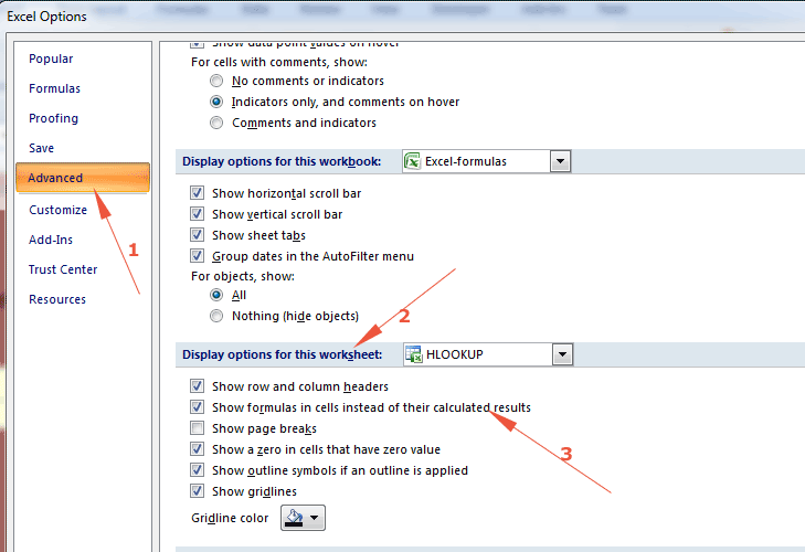
Press Ok.
Do the same steps for other worksheets that you want to display the formulas.