INDEX Function in Excel
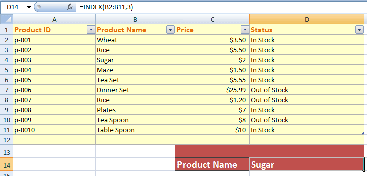
The Excel INDEX function requires the position and range and returns the value based on that position. If you do not know the position, you may get this by using MATCH function.
The Excel INDEX function requires the position and range and returns the value based on that position. If you do not know the position, you may get this by using MATCH function.
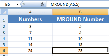
For getting the nearest multiple for any number like 5, 10, 100 etc. you may use the MROUND function in Excel. The MROUND function takes two arguments: MROUND(number, multiple)
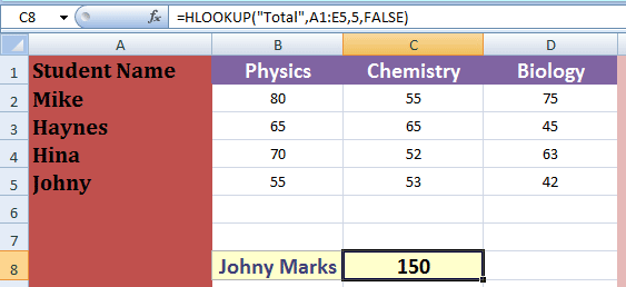
The Horizontal lookup function, HLOOKUP in excel is used to find the specific value in a row for the table that is arranged horizontally.
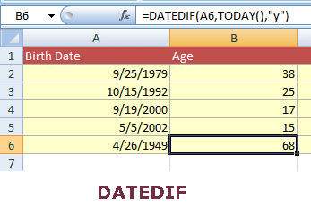
The Excel DATEDIF function takes the start date, end date, unit and calculates the difference in terms of days, months or years between these two dates. The unit specifies what you require; days, month, or years.
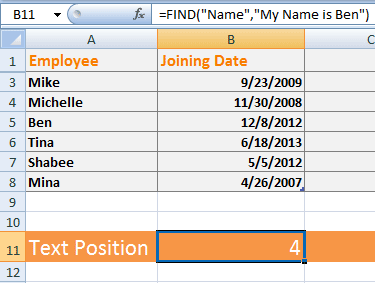
The FIND is case sensitive to return the position. The ‘C’ and ‘c’ has different meanings if you use FIND method to get the position of text in source string. The SEARCH function is case-insensitive. You may not use the ‘*’ and ‘?’ wildcards in the FIND function.
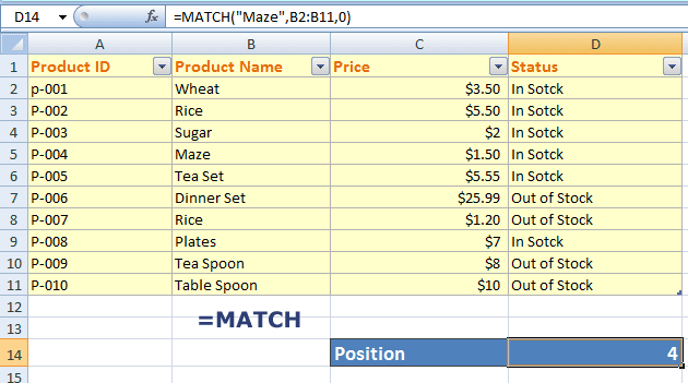
The Excel MACTH function returns the relative position of the specified item from the given range of cells. This is how the MATCH function can be used:
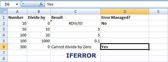
The IFERROR function enables us to trap and handle the errors that occur in functions or use it independently. You may display descriptive messages e.g. “0 is not allowed” etc.
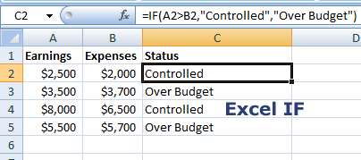
The IF statement is generally taken as a decision making statement. In Excel, the IF is a function that enables us doing that.
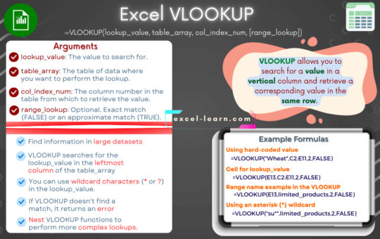
the VLOOKUP in Excel is used to “look up” or find a value in a table. The V in VLOOKUP function stands for Vertical. That means the VLOOKUP function works for data organized vertically.
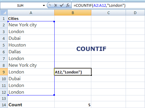
Use the Microsoft Excel COUNTIF function (a statistical function) that is used to count the number of cells for the given criterion.


