How to freeze panes in Excel?

Freezing the rows or columns while working in a long workbook can be really useful. For example, the top row contains the headers of the workbook and while entering data or analyzing it, you may lose the focus that what record belongs to which header.

To keep certain row or column, especially the top row or left column always in front of you can be achieved by using the “Freeze Panes” feature of MS Excel.

In this tutorial, I will show you the ways of freezing the panes; top row, any other row, and column etc. with screenshots and simple steps.

Where Freeze Panes option is located?

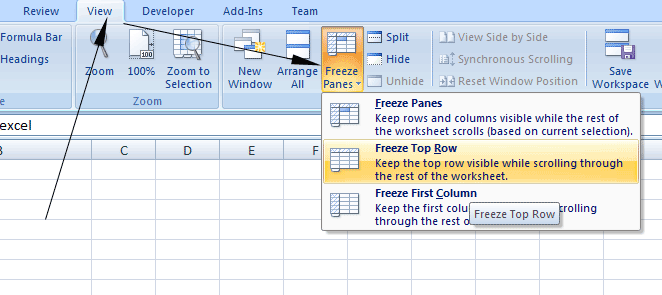
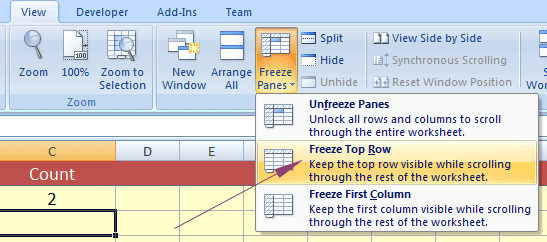
In MS Excel, press the “View” in the ribbon (top menu bar) and find the “Freeze Panes” icon in the toolbar as shown in the graphic below:

What is the shortcut of freezing panes?

For locking the cells or panes, you may use the following shortcut form the keyboard:

After selecting the cell, press:

Alt + W + F + F

For unfreezing the panes:

Select and press the

 Alt + W + F + F

The shortcuts for freezing the top row and left column are given below with their examples.

Freeze the top row example

Generally, it’s the top row that you would like to freeze in order to keep the headings in view all the time.

For fixing or freezing the top row, follow these simple steps:

Step1:

No need to select the row, just go to the “View” menu in the ribbon.

Step2:

Locate the “Free Panes” icon and open its menu and press the “Freeze Top Row” option as shown below:

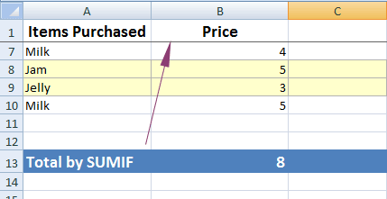
MS Excel should show a dark grey line that indicates the frozen pane. See the image below:

Unlocking the top row

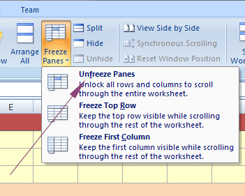
If the top row is locked then again go to the View and free panes button. As you open its menu, you should now see “Unfreeze Panes”. Press this button and top row should be unfrozen.

Using the shortcut for freezing the top row

Use the following shortcut:

Alt + W + F + F + R

For unfreezing the top row:

Alt + W + F + F

How to fix the first column example

Similarly, your headings may be contained in the left or first column of the workbook. In order to freeze the first column, follow this:

Step 1:

Go the “View” menu in the ribbon.

Step 2

Locate the “Freeze Panes” button and open its menu.

Step 3:

Press the “Freeze First Column” menu item as shown below:

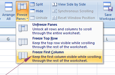
An example sheet is shown below with the first column frozen:

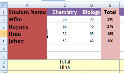
You can see, the A column is appearing and the next column is C as I scrolled to the next column. The B is disappeared while A column is still in the view.

The shortcut of making the first column frozen:

Alt + W + F + C

Unfreezing the first column

Just like unfreezing the cells and top row in the above examples, for unfreezing the first column, again go to “View” and select Unfreeze Panes under the Freeze Panes button.

Locking both top row and first column

In order to freeze both top row and first column at the same time, you may press the:

Freeze Top Row

and

Freeze First Column

One by one and this should fulfill the task. However, Excel will unfreeze both simultaneously if you press the “Unfreeze Panes” after freezing both.

How to fix multiple rows example

If you want to freeze not only the top row but subsequent rows as well, then follow this.

Suppose we want to fix till row number 4.

Step 1:

Select the row number 5.

Step 2:

Go to the View tab and press “Freeze Panes” and press the Freeze Panes option. You may also use the shortcut key i.e.

Alt + W + F + F

See an example sheet below:

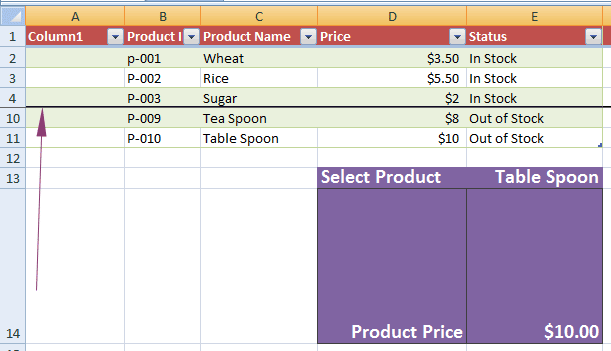
In the above graphic, you can see the row numbers 1,2,3,4 are appearing and the next row is 10 as I scroll down to that row.

Can I freeze single cell within?

No, Excel does not give the option to freeze a single or range of cells somewhere in between. For example, fixing the Grand Total etc.

For that, you may use an odd feature called the “Camera Tool”. This creates a floating picture of a cell’s value that you may put anywhere.